Implicit solution of 1D nonlinear porous medium equation using the four-point Newton-EGMSOR iterative method
J.V.L. Chew
,J. Sulaiman
Journal of Applied Mathematics and Computational Mechanics |
 Download Full Text |
IMPLICIT SOLUTION OF 1D NONLINEAR POROUS MEDIUM EQUATION USING THE FOUR-POINT NEWTON-EGMSOR ITERATIVE METHOD
J.V.L. Chew, J. Sulaiman
Faculty of Science and Natural Resources,
University Malaysia Sabah
Sabah, Malaysia
jackelchew93@gmail.com, jumat@ums.edu.my
Abstract. The numerical method can be a good choice in solving nonlinear partial differential equations (PDEs) due to the difficulty in finding the analytical solution. Porous medium equation (PME) is one of the nonlinear PDEs which exists in many realistic problems. This paper proposes a four-point Newton-EGMSOR (4-Newton-EGMSOR) iterative method in solving 1D nonlinear PMEs. The reliability of the 4-Newton-EGMSOR iterative method in computing approximate solutions for several selected PME problems is shown with comparison to 4-Newton-EGSOR, 4-Newton-EG and Newton-Gauss-Seidel methods. Numerical results showed that the proposed method is superior in terms of the number of iterations and computational time compared to the other three tested iterative methods.
Keywords: porous medium equation, finite difference scheme, Newton method, Explicit Group, MSOR
1. Introduction
Most of the nonlinear partial differential equations (PDEs) are difficult to be solved by the analytical approach. Since the rapid advancement of computers, numerical methods have grown drastically to be the choice in solving nonlinear PDEs. This paper considers a numerical approach for the solution of one of the nonlinear PDEs which is a porous medium equation (PME). This equation has great practicality in many realistic problems such as a thin film flow through a porous medium [1], diffusion of heat beneath human skin [2] and some interesting applications such as the dispersion of miscible fluid through a porous medium [3, 4] and the instability phenomena in the oil recovery technology [5-7]. Currently, the last two applications have been widely studied for the development of a theoretical model and finding the approximate analytical solution to the developed model. For instance, Meher et al. [3, 4] have discussed the dispersion phenomena inside porous media that occurs in oil reservoir and applied the Adomian decompo- sition method and the Backlund transformation in obtaining the analytical solutions of the problems. Meher et al. [5, 6] have applied the Adomian decomposition method and the exponential self similar solutions technique in solving PME which is formulated from the instability phenomena in double phase flow through porous media. In fact, there is much literature involving the solution of PME problems that can be found in [7-12]. Motivated and inspired by the ongoing research in solving PME, this paper proposes a four-point Newton-EGMSOR (4-Newton-EGMSOR) iterative method in solving 1D nonlinear PMEs. Actually, the method is a combination of four-point EGMSOR iteration which is initiated by Sulaiman et al. [13] with the Newton method that is used to handle the nonlinearity of the problem. This paper dealt with an efficient numerical technique that can reduce the computational time while maintaining the accuracy of the approximate solution of PMEs.
In this paper, to secure computational stability, a PME approximation equation is developed by using the implicit finite difference scheme. A system of nonlinear equations is formed at each time level. The Newton method is then used to linearize and transform the developed system of nonlinear equations into the corresponding system of linear equations. The resultant linear system is finally solved by the four-point EGMSOR iterative methods. Four examples of the PMEs are chosen in order to illustrate the capability of the 4-Newton-EGMSOR iterative method. The reliability of the proposed method in computing approximate solutions for the selected PME problems is shown with comparison to 4-Newton-EGSOR, 4-Newton-EG and Newton-Gauss-Seidel (GS) iterative methods. Consider a general form of the PME problem be defined as
| (1) |
where K and m are real numbers.
Solution domain x can be divided uniformly into d subintervals with distance Dx. Time step Dt can also be obtained by dividing the total time T at fixed sizes of s. Both steps, Dx and Dt, can be defined as
| (2) |
2. Implicit finite difference approximation equation
To formulate 4-Newton-EGMSOR for solving Eq. (1), a finite grid network is built as a guide for development of the three iterative methods and facilitating the implementation of computational algorithm, refer Figure 1.
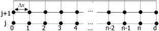
Fig. 1. Finite grid network
The implementation of the 4-Newton-EGMSOR method will be applied onto the interior grid points in Figure 1, i.e. grid point 1 to n, until the convergence of approximate solutions is achieved. Before discretizing, problem (1) can be rewritten as
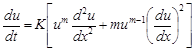 | (3) |
Now, by using the implicit finite difference scheme, (3) is discretized to derive an approximation equation as
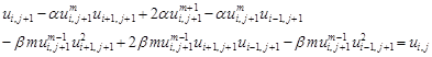 | (4) |
for i = 1, 2, 3, ..., n and j = 0,1, 2, 3, ..., s, where
Eq. (4) is obviously a nonlinear finite difference approximation equation that is used to form a system of nonlinear equations at each time level j. To apply the Newton method on Eq. (4), define a nonlinear function F for each interior grid point (xi , tj+1) at time level tj+1 as follows:
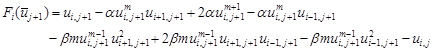 | (5) |
where ![]() .
.
By considering all interior grid points in Figure 1, Eq. (5) leads to nonlinear system as
| (6) |
Now, the Newton method can be used to calculate the Jacobian matrix on (6) in order to construct the corresponding linear system. Indicated with k-th numerical solutions at each time level tj+1, Eq. (6) is transformed into a linear system as
| (7) |
where
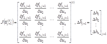 |
The unknown vector ![]() is required to be solved so
that the vector of approximate solutions
is required to be solved so
that the vector of approximate solutions ![]() can
be computed iteratively by using the following expression:
can
be computed iteratively by using the following expression:
| (8) |
3. Formulation and implementation of the four-point EGMSOR method
As discussed in the second section, the coefficient matrix A in linear system (7) is sparse and large-scaled, and therefore needs an efficient iterative method to be solved. A number of iterative methods can be found in [14-17]. In addition to that, Evans [18] has proposed a four-point block iterative method which is also known as Explicit Group (EG) in solving large linear systems. Again, the Successive Over Relaxation (SOR) method was introduced by Young [15] and it is the most known and widely used iterative technique in solving a system of linear algebraic equations. Due to the advantage of the SOR method, Kincaid and Young [17] have suggested Modified Successive Over Relaxation (MSOR) method, which is classified as a point iterative method together with two weighted parameters, wr and wb, in order to speed up the rate of convergence in SOR. Therefore, this paper considers the application of the four-point EGMSOR iterative method for solving the generated linear system and this iterative method is a combination between the EG and MSOR methods. Before formulating the four-point EGMSOR iterative method, let the linear system in (7) be rewritten in general form as
| (9) |
where
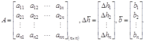 |
Now, the coefficient
matrix![]() in Eq. (9) needs to be decomposed as
in Eq. (9) needs to be decomposed as
| (10) |
where D, L and V are the diagonal, lower triangular part and upper triangular part of matrix A, respectively. Then, the formulation of the SOR method is given by [15]
| (11) |
When w = 1, the SOR method can be reduced to the standard GS iterative method. Apart from the concept of the SOR method, the MSOR methods can be derived from (11) with two weighted parameters, wr and wb. In fact, this concept is similar to the SOR method with the red-black ordering strategy. The formulation of the MSOR method is given by [17]
 | (12) |
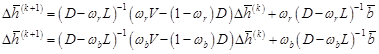
And then when wr = wb, the MSOR method reduces to the red-black SOR method. Besides that, by setting wr = wb = 1, (12) will become the red-black GS method. Since this paper uses four-point EGMSOR to solve the linear system that is transformed by using the Newton method, the derivation of four-point EGMSOR method will be constructed over the linear system (9) as follows.
Referring to Figure 1, a group of four points
is considered to be used to form
a linear system ![]() as
follows.
as
follows.
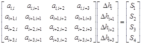 | (13) |
where
for t = 1, 2, 3, 4. Eq. (13) can be easily inverted and derived into a four-point EGMSOR formula that is similar to Eq. (12) as follows:
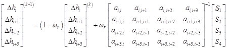 | (14a) |
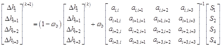 | (14b) |
Hence, by using Eqs. (14a) and (14b), the four-point EGMSOR algorithm can be given in Algorithm 1.
Algorithm 1. Four-point EGMSOR
i. Initialize ![]()
ii. For ![]() , implement
, implement
a. Set ![]()
b. Calculate ![]() , A and b
, A and b
c. For ![]() , compute Eq. (14a)
iteratively.
, compute Eq. (14a)
iteratively.
d. For ![]() , compute Eq. (14b)
iteratively.
, compute Eq. (14b)
iteratively.
e. For ![]() , compute ungroup
points. For more detail, see in [19].
, compute ungroup
points. For more detail, see in [19].
iii. Convergence test ![]() . If
converges, go to (iv). Otherwise, back to (ii).
. If
converges, go to (iv). Otherwise, back to (ii).
iv. Compute ![]()
v. Convergence test
![]() . If converges, go to next time level.
Otherwise, back to (i).
. If converges, go to next time level.
Otherwise, back to (i).
vi. Display approximate solutions.
The estimate values of the two weighted parameters are determined within range ± 0.01 by running Algorithm 1 with a different combination of wr and wb. The combination that gives the least number of iterations will be selected as optimal values.
4. Numerical experiments
In order to verify the effectiveness of 4-Newton-EGMSOR iterative method in solving (1), four selected PME problems are used together with other three tested iterative methods, i.e. 4-Newton-EGSOR, 4-Newton-EG and Newton-GS iterative methods, that act as comparison to the proposed iterative method. For the comparison purpose, three criteria will be considered, namely the number of iterations (Iter), execution time, which is measured in seconds (Time), and maximum absolute error (MAE). In addition to that, tolerance error for convergence is e = 10–10. Below is the following for four examples of PME problems.
Example 1 [19]
Consider K = 1 and m = 1 in (1) gives
| (15) |
subject to the
initial condition, ![]() , and satisfies the exact
solution,
, and satisfies the exact
solution, ![]() , where
, where ![]() and
and ![]() are arbitrary constants. For
the numerical implementation, constants are set to be
are arbitrary constants. For
the numerical implementation, constants are set to be ![]() and
and ![]() .
.
Example 2 [19]
Consider K = 0.5 and m = –1 in (1) gives
| (16) |
subject to the initial condition, ![]() , and satisfies the exact solution,
, and satisfies the exact solution, ![]() , where
, where ![]() and
and ![]() are
arbitrary constants. To implement the iterative methods, constants chosen are
are
arbitrary constants. To implement the iterative methods, constants chosen are
![]() and
and ![]() .
.
Example 3 [8]
Consider K = 1 and m = 2 in (1) gives
| (17) |
subject to the initial condition, ![]() , and
satisfies the exact solution,
, and
satisfies the exact solution, ![]() ,
, ![]() , where C is an arbitrary constant. For the imple-
mentation purpose, the constant is C = 2.
, where C is an arbitrary constant. For the imple-
mentation purpose, the constant is C = 2.
Example 4 [19]
Consider K = 0.5 and m = –2 in (1) gives
| (18) |
subject to the initial condition, ![]() , and satisfies the exact solu-
tion,
, and satisfies the exact solu-
tion, ![]() , where
, where ![]() and
and ![]() are arbitrary
constants. To test
the numerical methods, constants are set to be
are arbitrary
constants. To test
the numerical methods, constants are set to be ![]() and
and ![]() .
.
The numerical results obtained have been summarized in Tables 1-3.
Table 1
Comparison of the number of iterations (Iter), execution time in seconds (Time) and maximum absolute errors (MAE) for the iterative methods using Examples 1 and 2
|
|
|
Example 1 |
Example 2 |
||||||
|
n |
Method |
|
Iter |
Time |
MAE |
|
Iter |
Time |
MAE |
|
64 |
GS |
|
3835 |
2.38 |
2.76E-08 |
|
1720 |
1.13 |
2.03E-05 |
|
|
EG |
|
1109 |
0.34 |
5.88E-09 |
|
504 |
0.55 |
2.03E-05 |
|
|
EGSOR |
w = 1.59 |
263 |
0.12 |
3.43E-11 |
w = 1.47 |
175 |
0.25 |
2.03E-05 |
|
|
EGMSOR |
wr = 1.59 wb = 1.58 |
240 |
0.10 |
2.99E-11 |
wr = 1.47 wb = 1.48 |
147 |
0.16 |
2.03E-05 |
|
128 |
GS |
|
13 678 |
7.50 |
1.22E-07 |
|
6034 |
4.06 |
2.02E-05 |
|
|
EG |
|
3899 |
1.65 |
2.64E-08 |
|
1718 |
1.73 |
2.03E-05 |
|
|
EGSOR |
w = 1.76 |
513 |
0.34 |
4.28E-11 |
w = 1.68 |
337 |
0.41 |
2.03E-05 |
|
|
EGMSOR |
wr = 1.76 wb = 1.77 |
455 |
0.31 |
1.61E-11 |
wr = 1.68 wb = 1.69 |
275 |
0.38 |
2.03E-05 |
|
256 |
GS |
|
48 395 |
38.58 |
5.33E-07 |
|
20 907 |
27.03 |
2.00E-05 |
|
|
EG |
|
13 799 |
11.20 |
1.10E-07 |
|
5976 |
11.25 |
2.02E-05 |
|
|
EGSOR |
w = 1.87 |
1010 |
1.37 |
6.90E-11 |
w = 1.82 |
656 |
1.35 |
2.03E-05 |
|
|
EGMSOR |
wr = 1.87 wb = 1.88 |
879 |
1.20 |
3.62E-11 |
wr = 1.82 wb = 1.83 |
532 |
1.14 |
2.03E-05 |
|
512 |
GS |
|
169 693 |
252.94 |
2.10E-06 |
|
71 385 |
287.34 |
1.93E-05 |
|
|
EG |
|
48 666 |
77.31 |
4.99E-07 |
|
20 701 |
97.75 |
2.00E-05 |
|
|
EGSOR |
w = 1.93 |
2027 |
5.33 |
7.69E-10 |
w = 1.91 |
1297 |
4.46 |
2.03E-05 |
|
|
EGMSOR |
wr = 1.93 wb = 1.94 |
1680 |
4.51 |
4.23E-11 |
wr = 1.90 wb = 1.91 |
1050 |
3.82 |
2.03E-05 |
|
1024 |
GS |
|
587 031 |
1712.49 |
7.62E-06 |
|
239 975 |
1741.01 |
1.72E-05 |
|
|
EG |
|
170 300 |
557.86 |
2.08E-06 |
|
70 888 |
571.03 |
1.94E-05 |
|
|
EGSOR |
w = 1.97 |
4072 |
22.43 |
1.54E-10 |
w = 1.95 |
2477 |
24.67 |
2.03E-05 |
|
|
EGMSOR |
wr = 1.96 wb = 1.97 |
3417 |
19.72 |
1.18E-10 |
wr = 1.95 wb = 1.95 |
2078 |
22.87 |
2.03E-05 |
Table 2
Comparison of the number of iterations (Iter), execution time in seconds (Time) and maximum absolute errors (MAE) for the iterative methods using Examples 3 and 4
|
|
|
Example 3 |
Example 4 |
||||||
|
n |
Method |
|
Iter |
Time |
MAE |
|
Iter |
Time |
MAE |
|
64 |
GS |
|
1344 |
1.17 |
8.39E-05 |
|
2015 |
1.26 |
2.88E-06 |
|
|
EG |
|
402 |
0.38 |
8.39E-05 |
|
592 |
0.53 |
2.89E-06 |
|
|
EGSOR |
w = 1.35 |
216 |
0.13 |
8.39E-05 |
w = 1.49 |
191 |
0.30 |
2.90E-06 |
|
|
EGMSOR |
wr = 1.35 wb = 1.30 |
202 |
0.13 |
8.39E-05 |
wr = 1.49 wb = 1.49 |
165 |
0.17 |
2.90E-06 |
|
128 |
GS |
|
4824 |
2.84 |
8.39E-05 |
|
7082 |
4.90 |
2.90E-06 |
|
|
EG |
|
1361 |
1.00 |
8.39E-05 |
|
2033 |
1.85 |
2.94E-06 |
|
|
EGSOR |
w = 1.58 |
437 |
0.41 |
8.39E-05 |
w = 1.69 |
380 |
0.89 |
2.96E-06 |
|
|
EGMSOR |
wr = 1.59 wb = 1.54 |
405 |
0.36 |
8.39E-05 |
wr = 1.69 wb = 1.70 |
316 |
0.44 |
2.96E-06 |
|
256 |
GS |
|
17 308 |
20.03 |
8.39E-05 |
|
24 325 |
45.42 |
2.71E-06 |
|
|
EG |
|
4836 |
6.77 |
8.39E-05 |
|
7007 |
15.11 |
2.92E-06 |
|
|
EGSOR |
w = 1.74 |
873 |
1.47 |
8.39E-05 |
w = 1.83 |
734 |
1.98 |
2.97E-06 |
|
|
EGMSOR |
wr = 1.74 wb = 1.74 |
810 |
1.21 |
8.39E-05 |
wr = 1.83 wb = 1.84 |
609 |
1.42 |
2.97E-06 |
|
512 |
GS |
|
61 658 |
270.11 |
8.40E-05 |
|
81 729 |
354.79 |
1.86E-06 |
|
|
EG |
|
17 333 |
46.85 |
8.39E-05 |
|
23 769 |
112.83 |
2.73E-06 |
|
|
EGSOR |
w = 1.86 |
1718 |
5.38 |
8.38E-05 |
w = 1.91 |
1428 |
5.82 |
2.98E-06 |
|
|
EGMSOR |
wr = 1.87 wb = 1.86 |
1563 |
4.38 |
8.39E-05 |
wr = 1.91 wb = 1.91 |
1202 |
4.76 |
2.98E-06 |
|
1024 |
GS |
|
218 147 |
2008.35 |
8.43E-05 |
|
265 698 |
2293.23 |
3.33E-06 |
|
|
EG |
|
61 779 |
342.02 |
8.40E-05 |
|
79 057 |
733.85 |
1.89E-06 |
|
|
EGSOR |
w = 1.93 |
3344 |
20.49 |
8.39E-05 |
w = 1.95 |
2881 |
26.41 |
2.97E-06 |
|
|
EGMSOR |
wr = 1.93 wb = 1.92 |
3066 |
16.83 |
8.39E-05 |
wr = 1.95 wb = 1.96 |
2311 |
19.75 |
2.98E-06 |
Table 3
Reduction in percentages of the iterative methods compared with the GS method
|
M |
Method |
Number of iterations |
Execution time in seconds |
||||||
|
Example 1 |
Example 2 |
Example 3 |
Example 4 |
Example 1 |
Example 2 |
Example 3 |
Example 4 |
||
|
64 |
EG |
71.08% |
70.70% |
70.09% |
70.62% |
85.71% |
51.33% |
67.52% |
57.94% |
|
|
EGSOR |
93.14% |
89.83% |
83.93% |
90.52% |
94.96% |
77.88% |
88.89% |
76.19% |
|
|
EGMSOR |
93.74% |
91.45% |
84.97% |
91.81% |
95.80% |
85.84% |
88.89% |
86.51% |
|
128 |
EG |
71.49% |
71.53% |
71.79% |
71.29% |
78.00% |
57.39% |
64.79% |
62.24% |
|
|
EGSOR |
96.25% |
94.41% |
90.94% |
94.63% |
95.47% |
89.90% |
85.56% |
81.84% |
|
|
EGMSOR |
96.67% |
95.44% |
91.60% |
95.54% |
95.87% |
90.64% |
87.32% |
91.02% |
|
256 |
EG |
71.49% |
71.42% |
72.06% |
71.19% |
70.97% |
58.38% |
66.20% |
66.73% |
|
|
EGSOR |
97.91% |
96.86% |
94.96% |
96.98% |
96.45% |
95.01% |
92.66% |
95.64% |
|
|
EGMSOR |
98.18% |
97.46% |
95.32% |
97.50% |
96.89% |
95.78% |
93.96% |
96.87% |
|
512 |
EG |
71.32% |
71.00% |
71.89% |
70.92% |
69.44% |
65.98% |
82.66% |
68.20% |
|
|
EGSOR |
98.81% |
98.18% |
97.21% |
98.25% |
97.89% |
98.45% |
98.01% |
98.36% |
|
|
EGMSOR |
99.01% |
98.53% |
97.47% |
98.53% |
98.22% |
98.67% |
98.38% |
98.66% |
|
1024 |
EG |
70.99% |
70.46% |
71.68% |
70.25% |
67.42% |
67.20% |
82.97% |
68.00% |
|
|
EGSOR |
99.31% |
98.97% |
98.47% |
98.92% |
98.69% |
98.58% |
98.98% |
98.85% |
|
|
EGMSOR |
99.42% |
99.13% |
98.59% |
99.13% |
98.85% |
98.69% |
99.16% |
99.14% |
5. Conclusion
In this paper, the effectiveness of the 4-Newton-EGMSOR in solving 1D non-linear PMEs as compared with other three tested iterative methods, i.e. 4-Newton-‑EGSOR, 4-Newton-EG and Newton-GS iterative methods, have been demonstrated by using four PME problems. The numerical results presented in Tables 1 and 2 showed that the proposed iterative method requires a much lesser number of iterations and computational time in obtaining numerical solutions as compared to the other three tested iterative methods. By using the Newton-GS as a control method, 4-Newton-EGMSOR has a reduced number of iteration of approximately 84.97- ‑99.42% and computational time approximately 85.84-99.16%, see in Table 3. The performance showed by the 4-Newton-EGMSOR is aided by the use of two weighted parameters, wr and wb. When these two weighted parameters achieved their optimal choices, the maximum speed of convergence in solving the PME problems can be reached. And in terms of the accuracy of the iterative methods, all four tested numerical methods have good agreement. Therefore, it can be concluded that the 4-Newton-EGMSOR iterative method can be a promising technique for solving different types of nonlinear partial differential equation problems. In this paper, however, all four iterative methods can be classified under a family of full-sweep iterative methods. Hence, for future work, this study will be extended for a family of half-sweep iterative methods [21-24].
References
[1] Mahmood T., Khan N., Thin film flow of a third grade fluid through porous medium over an inclined plane, International Journal of Nonlinear Science 2012, 14(1), 53-59.
[2] Khaled A.R.A., Vafai K., The role of porous media in modelling flow and heat transfer in biological tissues, International Journal of Heat and Mass Transfer 2003, 46, 4989-5003.
[3] Meher R., Mehta M.N., Meher S.K., Adomian decomposition method for dispersion phenomena arising in longitudinal dispersion of miscible fluid flow through porous media, Advances in Theoretical and Applied Mechanics 2010, 3(5), 211-220.
[4] Meher R.K., Meher S.K., Mehta M.N., A new approach to Backlund transformation for longitudinal dispersion of miscible fluid flow through porous media in oil reservoir during secondary recovery process, Theoretical and Applied Mechanics 2011, 38(1), 1-16.
[5] Meher R.K., Meher S.K., Analytical treatment and convergence of the Adomian decomposition method for instability phenomena arising during oil recovery process, International Journal of Engineering Mathematics 2013, Article ID-752561.
[6] Meher R.K., Meher S.K., Mehta M.N., Exponential self similar solutions technique for instability phenomenon arising in double phase flow through porous medium with capillary pressure, Applied Mathematics Sciences 2010, 4(27), 1329-1335.
[7] Pradhan V.H., Mehta M.N., Patel T., A numerical solution of nonlinear equation representing one-dimensional instability phenomena in porous media by finite element technique, Inter- national Journal of Advanced Engineering Technology 2011, 2(1), 221-227.
[8] Elsheikh A.M., Elzaki T.M., Variation iteration method for solving porous medium equation, International Journal of Development Research 2015, 5(6), 4677-4680.
[9] Wazwaz A.M., The variational iteration method: A powerful scheme for handling linear and nonlinear diffusion equations, Computers and Mathematics with Application 2007, 54, 933-939.
[10] Bhadane P.K.G., Pradhan V.H., Elzaki transform homotopy pertubation method for solving porous medium equation, International Journal of Research in Engineering and Technology 2013, 2(12), 116-119.
[11] Elzaki T.M., Hilal E.M.A., Homotopy perturbation and Elzaki transform for solving nonlinear partial differential equations, Mathematical Theory and Modeling 2012, 2(3), 33-42.
[12] Pamuk S., On the solution of the porous media equation by decomposition method: A review, Physics Letters A 2005, (344), 184-188.
[13] Sulaiman J., Hasan M.K., Othman M., Karim S.A.A., Newton-EGMSOR methods for solution of second order two-point nonlinear boundary value problems, Journal of Mathematics and System Science 2012, 2, 185-190.
[14] Saad Y., Iterative Methods for Sparse Linear Systems, 2nd ed., Society for Industrial and Applied Mathematics, Philadelphia 2003.
[15] Young D.M., Iterative methods for solving partial difference equations of elliptic type, Transactions of the American Mathematical Society 1954, 76, 92-111.
[16] Young D.M., Iterative Solution of Large Linear Systems, Academic Press, Florida 2014.
[17] Kincaid D.R., Young D.M., The modified successive over relaxation method with fixed parameters, Mathematics of Computation 1972, 26(119), 705-717.
[18] Evans D.J., Group explicit iterative methods for solving large linear systems, International Journal of Computer Mathematics 1985, 17, 81-108.
[19] Evans D.J., Abdullah A.R., A new explicit method for the diffusion-convection equation, Computers and Mathematics with Applications 1985, 11, 1-3.
[20] Polyanin A.D., Zaitsev V.F., Handbook of Nonlinear Partial Differential Equation, Chapman and Hall, Boca Raton 2004.
[21] Akhir M.K.M., Othman M., Sulaiman J., Majid Z.A., Suleiman M., Half-sweep modified successive over relaxation for solving two-dimensional Helmholtz equations, Australian Journal of Basic and Applied Sciences 2011, 5(12), 3033-3039.
[22] Othman M., Sulaiman J., Abdullah A.R., A parallel halfsweep multigrid algorithm on the shared memory multiprocessors, Malaysian Journal of Computer Science 2000, 13(2), 1-6.
[23] Muthuvalu M.S., Sulaiman J., Half-sweep geometric mean method for solution of linear Fredholm equations, Matematika 2008, 24(1), 75-84.
[24] Aruchunan E., Sulaiman J., Half-sweep conjugate gradient method for solving first order linear Fredholm integro-differential equations, Australian Journal of Basic and Applied Sciences 2011, 5, 38-43.