Remarks on the impact of the adopted scale on the priority estimation quality
Tomasz Starczewski
Journal of Applied Mathematics and Computational Mechanics |
 Download Full Text |
REMARKS ON THE IMPACT OF THE ADOPTED SCALE ON THE PRIORITY ESTIMATION QUALITY
Tomasz Starczewski
Institute of Mathematics, Czestochowa
University of Technology
Czestochowa, Poland
starczewski.t@gmail.com
Received: 5 June 2017; Accepted: 11 September 2017
Abstract. The Analytic Hierarchy Process (AHP) is the method that supports people’s decisions in the multi-criteria decision making problems. In this method the decision process is based on pairwise comparing of every two possible alternatives. The decision maker (DM) compares alternatives by choosing an appropriate “linguistic phrase” or a number from a proper set. This set of “linguistic phrases” and/or the numbers connected with them are referred to as the priority scale. There are several different scales that are described in literature and used in AHP practice. In dependence of the scale chosen by the DM, the final decisions might differ. In the AHP it is assumed that DMs make mistakes over comparing pairs of alternatives, but it was also observed that the assumed scale increases these errors as well. In our paper, we investigate the impact of the adopted scale to the number and magnitude of errors in the final decision. Our results show that the choice of the scale has a big impact on the final decision, so it is crucial part of AHP. It turns out that scales with bigger resource of options result in better evaluations of priority vectors.
MSC 2010: 15B52, 62C07, 62C86, 90B50, 91B06
Keywords: Analytic Hierarchy Process (AHP), priority scale, pairwise comparison
1. Introduction - scale in AHP
The Analytic Hierarchy Process (AHP) is the method which supports people’s decisions. The decisions often consist of the best alternative choice from the possible alternatives. In the AHP, the decision maker (DM) answers the question in order to compare every two among all alternatives in respect to any criterion. DM answers the questions: "Which alternative: A or B do you prefer?" and "How much do you prefer this alternative?". In this way, the pairwise comparison matrix (PCM) arises. In this matrix, the element in i-th raw and j-th column says how much more (or less) DM prefer i-th over j-th alternative [1].
PCM consists of numbers which correspond to DM’s answers about his (i.e. the DM’s) judgments about the preference ratios. However, DM’s answers are expressed in "linguistic values" and not directly in a numerical value. So we need convert the answers in common language to numbers. For this purpose, the priority scale is used. T. Saaty introduced such a scale, called Fundamental Scale (FS) [1]. It is based on 9 natural numbers and its reciprocals which are connected with certain linguistic expressions. Despite some negative opinions of using FS, see [2-4], it is the most popular scale adopted in the AHP practice.
Apart from the FS we investigate two other scales: the extension of FS to the larger set of the natural number scale which we call the Extension Scale (ES) and the Geometric Scale (GS) [4], which is a little less popular than FS but also often encountered in literature. The ES is similar to the FS but makes it possible to compare more different alternatives without dividing them into classes (an idea of Saaty [1]) and obtaining a more actual estimate of PCM elements. The numbers in GS, in difference to FS, can be interpreted as actual ratios between related linguistic expressions. An interesting case, which we investigate in this paper, is the case without scale. Obviously, it is a case which cannot be observed in practice but its investigating helps us to find out more information about the impact of assumed scales on the final decisions quality.
In common AHP practice, the DM compares every pair of alternatives with respect to any criterion only one time (if you compare A to B you do not have to compare B to A). It is due to opinion that reliable DM gives reciprocals answer when he compares A with B and B with A. So, to ensure reciprocity PCM obtained from questionnaire numbers are entered in upper triangle PCM and next the lower triangle is filled with the reciprocals of elements from the upper triangle. However in practice the DM often gives nonreciprocal answers, so in our paper we consider both cases: reciprocal and nonreciprocal matrices (more opinions: [2, 5-9]).
As we mentioned, the principal aim of AHP is ordering the alternatives. For this purpose, one should evaluate the priority weights, i.e. numbers which indicate relative importance of given alternatives with respect to given criterion. The priority weights form a vector that we call the priority vector (PV). In the literature, some methods were introduced that can be used to estimate the PV from a given PCM (see e.g. [9-12]). The two most frequently used methods are Right Eigenvector Method, ([1, 12]) and Row Geometric Mean Procedure (GM) ([11]). Each prioritization method allow to derive the true PV from PCM if the PCM has no errors. However such a case is not possible in the practice because of the influence of many circumstances, which in the theory are expressed as a random factor ([10, 13]). In our paper we use the GM because this method is relatively easy to apply and it makes possible to obtain the PV from both, reciprocal and nonreciprocal PCMs. For more discussions about deriving the PVs from the PCMs see [5, 7, 9, 14, 15].
The aim of our paper is to analyse the dependence of the quality of the final decisions about priority vectors on the assumed scale that expresses the pairwise comparisons judgments. To achieve this purpose, we investigate three of the most popular scales which will be described in the next chapter.
2. Preliminaries - AHP
The main goal of the AHP is ordering
alternatives regarding to the criteria. It is achieved by estimation of the PV,
that is an ![]() -dimensional vector
-dimensional vector
| (1) |
whose components ![]() , are the alternatives’
priority weights (priorities).
, are the alternatives’
priority weights (priorities).
2.1. Fundamental definitions
In this section we list the basic definitions which are important to understand our investigations.
Definition 1
The PCM
is a matrix ![]() whose elements
whose elements ![]() are DM judgments about real priority ratios
are DM judgments about real priority ratios ![]() .
.
Because ![]() are DM judgment about true value of ratio, so we assume influence
of random factor
are DM judgment about true value of ratio, so we assume influence
of random factor ![]() . Thus it holds [9-11]:
. Thus it holds [9-11]:
| (2) |
where ![]() is random variable called a random factor (RF) with any
distribution with expected value equal to 1.
is random variable called a random factor (RF) with any
distribution with expected value equal to 1.
As we mentioned in introduction, in this paper we estimate the PV from the given PCM by using the GM:
Definition 2
To estimate components of the PV on the basis of the
given ![]() one can use formula [6]:
one can use formula [6]:
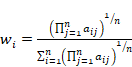 | (3) |
The vector ![]() is the estimate of the true PV, that will be called the priority-vector-estimate
(PVE).
is the estimate of the true PV, that will be called the priority-vector-estimate
(PVE).
Definition 3
A given PCM
matrix ![]() is called reciprocal if the following condition holds:
is called reciprocal if the following condition holds:
| (4) |
for any i, j =1,2,…,n [2].
2.2. Errors
The obtained according to formula (3) PV elements might contain errors. However, we do not know the true PV, so the errors in practice are impossible to observe. In the conducted research, we assume initial value of PV to be known, and next assume randomly generated values of RF in order to simulate “real” disturbed-PCM. From disturbed-PCM we obtain PVE, which is unfailingly different from the true PV.
Definition 4
If we know the true PV and we obtain the disturbed PVE according to GM (or any other prioritization method) we can calculate the relative error (RE) [2] of PVE according to formula:
| (5) |
where ![]() are elements of PV and
are elements of PV and ![]() are elements of PVE.
are elements of PVE.
Definition 5
Assume that sorted PV
is equal ![]() and assume that
and assume that ![]() is the
order number of corresponding alternative. Assume that not sorted PVE is equal
is the
order number of corresponding alternative. Assume that not sorted PVE is equal ![]() where
where ![]() corresponds to the same alternative as
corresponds to the same alternative as
![]() . If there exists such
. If there exists such ![]() that
that ![]() and
and ![]() we say that there exist the
ordering error (OE) in PVE.
we say that there exist the
ordering error (OE) in PVE.
Because OEs appear when changes in order of alternatives priority occur so they mean, that the DM makes wrong decision. Sometimes the differences between changed alternatives priority are slight or insignificant. Because of that, in our paper, we introduced the next “measure” of PV errors.
Definition 6
Serious ordering
error (SOE) is an OE wherein inequality ![]() is held by such an alternative which also
hold inequality
is held by such an alternative which also
hold inequality ![]() where
where ![]() is a certain fixed positive real value, which is a
threshold for admissible errors in ordering.
is a certain fixed positive real value, which is a
threshold for admissible errors in ordering.
2.3. Scales
As we mentioned in Introduction, in real AHP
practice, the PCM is received
after transform answers of the DM to the numbers. Each component of PCM is
a number corresponding to answer: "How much better is it for you ![]() -th
alternative than
-th
alternative than ![]() -th regarding certain
criterion?". However, the answer is any phrase, not a number, which
the DM chooses from a set of some possible options. Obviously, there is limited
amount of possible answers which are assigned to limited amount of possible
values in the PCM. The set of possible different values in the PCM (i.e.
possible options for the answers) are defined by scales. In our paper we
consider three scales known from literature.
-th regarding certain
criterion?". However, the answer is any phrase, not a number, which
the DM chooses from a set of some possible options. Obviously, there is limited
amount of possible answers which are assigned to limited amount of possible
values in the PCM. The set of possible different values in the PCM (i.e.
possible options for the answers) are defined by scales. In our paper we
consider three scales known from literature.
The most popular scale called the FS, introduced by T. Saaty [1] consists of 9 natural numbers and theirs reciprocals:
| (6) |
T. Saaty proposed the following phrase to number assignment for expressing preferences:
1 - Equal importance
2 - Weak or slight more important
3 - Moderate more important
4 - Moderate plus more important
5 - Strong more important
6 - Strong plus more important
7 - Very strong or demonstrated more important
8 - Very, very strong more important
9 - Extremely more important
The reciprocals of these numbers are assigned when alternatives are respectively less important.
It is obvious that the necessity of using a
bigger quantity of numbers sometimes may occur, for example, because of a big
number of alternatives between which quite big or quite slight importance
differences occur. T. Saaty proposed in this case dividing all alternatives in
some comparatively equal importance groups [1]. This approach may be quite
problematic and make a difficult investigation of this scale. So, here we
propose similar scale with more possible options. Namely, we assume scale that consists of 50 natural numbers and its
reciprocals, which we call ![]() :
:
| (7) |
This scale was used by other researches as the reasonable approximation to the unconstrained situation in which the DM select any real number to express his judgment [5]. Indeed it is significantly richer than FS so it is much closer to the case without any scale.
The next scale, we take into account, is GS,
see [6]. As opposed to the previous scales consisting of a succeeding natural
numbers and theirs reciprocals, this scale consists of number which creates
geometric sequence. The original GS consists of 9 succeeding powers of number 2.
However, we decrease the interval between next powers from ![]() to
to ![]() and
we assumed a scale consists of the powers from 0 to 4 of number
and
we assumed a scale consists of the powers from 0 to 4 of number ![]() . We
adopted the symbol
. We
adopted the symbol ![]() for GS consist of succeeding
for GS consist of succeeding ![]() powers with interval
powers with interval ![]() of number
of number ![]() and their reciprocals. In our investigation, we consider
and their reciprocals. In our investigation, we consider ![]() :
:
| (8) |
We choose the number ![]() as
the base number in this scale, because in such a case there are not very big
differences for positive powers and not very small differences between negative
powers. Such a base number results in more precision rounding for small
differences between alternatives’ priorities. It is our novel approach to GS
(see [4]).
as
the base number in this scale, because in such a case there are not very big
differences for positive powers and not very small differences between negative
powers. Such a base number results in more precision rounding for small
differences between alternatives’ priorities. It is our novel approach to GS
(see [4]).
Because the GS is the geometric sequence, so a ratio of two succeeding options from GS is always the same. In our case the answer for two next priorities of alternative is that one is 10% more important than the other. So, it is clear that the GS has natural interpretation and there is no problem with transforming the DM judgment about priority ratios into numbers.
3. Simulation and result
In the previous sections we introduced
notions which are used in the AHP. The main issue which interests us in this
article is the impact of the adopted scales for the quality of the decision in
the AHP. The natural indicators of scale properties are values of errors
appearing in PVE when we use particular scales. In our paper, we calculate
values of RE with formula (5) and frequency of appearing error-values in
ordering PV, i.e. frequency of OEs and SOEs. For SOEs we assume the threshold ![]() . We
observe the amount of these errors in relation to the adopted scales, PCM
reciprocity, and size of standard deviation (SD). In part of the simulations we also assumed one big
disturbing error, which is multiplication of one chosen
element of PCM by number 2 or 3. It is simulation of outsized mistakes which
sometimes appear among the DM’s judgments. Our Monte Carlo Simulation approach
is based on the idea introduced in [2, 10]. Such an approach was also adopted
in several other papers, see e.g. [9, 13-16].
. We
observe the amount of these errors in relation to the adopted scales, PCM
reciprocity, and size of standard deviation (SD). In part of the simulations we also assumed one big
disturbing error, which is multiplication of one chosen
element of PCM by number 2 or 3. It is simulation of outsized mistakes which
sometimes appear among the DM’s judgments. Our Monte Carlo Simulation approach
is based on the idea introduced in [2, 10]. Such an approach was also adopted
in several other papers, see e.g. [9, 13-16].
3.1. Simulation frameworks
In order to obtain a value of RE in PVE for different scale, we perform the Monte Carlo simulation experiment that consists of following steps:
1.
Randomly generate ![]() -dimensional
PV (1).
-dimensional
PV (1).
2.
Generate ideal matrix of true priority ratios
according to formula ![]() .
.
3. Disturb the elements of the ideal matrix with formula (2) with certain probability distribution of PF and mark the new disturbed matrix as PCM.
4. Randomly select one element from the upper triangle of PCM and multiple them by big factor (BF).
5. Round the components of PCM to the nearest number of the examined priority scale (one of introduced in 2.3).
6. Force the reciprocal (in the reciprocal case) by replacement the elements from the lower triangle of PCM on reciprocals of elements from upper triangle accordance to formula (4).
7. Calculate elements PVE from PCM in accordance to formula (3).
8. Calculate RE between PV and PVE (5).
9.
Check alternatives ordering in PVE and PV and
mark every case with OE ![]() ) or without OE (
) or without OE (![]() ) (def. 5).
) (def. 5).
10. In case ![]() , check the differences in PV between turned alternatives and mark
every case with SOE (
, check the differences in PV between turned alternatives and mark
every case with SOE (![]() ) or without SOE (
) or without SOE (![]() ) respectively (def. 6); every case without OE is marked
) respectively (def. 6); every case without OE is marked ![]() .
.
11. Record the obtained value of errors in database.
12. Repeat steps 3-11 for ![]() different disturbances (
different disturbances (![]() times).
times).
13. Repeat steps 1-12 for 100 different PVs (100 times).
We run the above simulation for 4 probability
distribution families of PF (step 3): Normal, Gamma, Logarithm Normal and
Uniform. Each of them we adopted with 3 different values of SD: ![]() and
with expected value always equal 1. As it was proved [11], the choice of the
distribution family is not important so we prepared our simulation with mixed
family distribution.
and
with expected value always equal 1. As it was proved [11], the choice of the
distribution family is not important so we prepared our simulation with mixed
family distribution.
In step 4, one big error is introduced to the
PCM. We run simulation for 3 different values of BF:1, 2, 3, where case ![]() is actually a case without a big
error. For a different values of BF, we obtain different results, which we
record in database.
is actually a case without a big
error. For a different values of BF, we obtain different results, which we
record in database.
We run the above calculation separately for the 3 priority scale introduced in subsection 2.3, as well as without rounding to any scale. In the case without rounding to scale the step 5 is omitted.
We run the same calculation for both cases: reciprocal (with step 6) and nonreciprocal (without step 6).
Although we run simulation for ![]() , to
save the article space we present the results only for
, to
save the article space we present the results only for ![]() .
The results obtained for
.
The results obtained for ![]() are very similar to below presented results.
are very similar to below presented results.
The selected results are presented in Tables 1-6 in the next subsection. They are rounded to the 2nd decimal place. In each table, there are collected results of errors in PVE obtained from disturbed PCM by PF with 3 values of standard deviations and with different adopted Scales for both: reciprocal and nonreciprocal cases.
3.2. Result describing
In Table 1 there are collected values of mean
RE in PVE. As you might expect, the smallest values are in the column with the
results related to not rounded (to scale) PCM. The values obtained in this case
are within the range 0.03-0.10 for the nonreciprocal PCMs, and 0.04-0.12 for
the reciprocal matrices. We obtained slightly bigger values of RE for ![]() , but the differences are not big and balance
at 0.01-0.02. Slightly bigger differences occur between
, but the differences are not big and balance
at 0.01-0.02. Slightly bigger differences occur between![]() and FS which are up 0.04-0.07. However, the values of error for FS
do not exceed 0.15 for reciprocal PCMs, and 0.17 for nonreciprocal matrices.
Moreover, they are about twice bigger than values for not rounded PCMs.
Surprisingly big errors are obtained for
and FS which are up 0.04-0.07. However, the values of error for FS
do not exceed 0.15 for reciprocal PCMs, and 0.17 for nonreciprocal matrices.
Moreover, they are about twice bigger than values for not rounded PCMs.
Surprisingly big errors are obtained for ![]() . They balance at 0.73-0.84 for the nonreciprocal and at 0.77-0.81
for the reciprocal matrices.
. They balance at 0.73-0.84 for the nonreciprocal and at 0.77-0.81
for the reciprocal matrices.
As one might expect, the smaller RE in PV are
gained for nonreciprocal matrix. This dependence is observed both in the case
without rounding to scale and with FS and ES scale. Only for ![]() for reciprocal matrix for some of SD average REs are smaller but
the differences are not big.
for reciprocal matrix for some of SD average REs are smaller but
the differences are not big.
Table 1
The average relative errors (RE) in PVEs obtained in simulations (sec. 3.1) without big errors: BF = 1
|
|
Nonreciprocal |
Reciprocal |
||||||
|
Scale: |
without |
FS |
ES(50) |
GS(1.2,0.5,9) |
without |
FS |
ES(50) |
GS(1.2,0.5,9) |
|
SD = 0.1 |
0.03 |
0.11 |
0.05 |
0.84 |
0.04 |
0.10 |
0.06 |
0.77 |
|
SD = 0.2 |
0.07 |
0.15 |
0.08 |
0.73 |
0.08 |
0.13 |
0.09 |
0.81 |
|
SD = 0.3 |
0.10 |
0.15 |
0.11 |
0.84 |
0.12 |
0.17 |
0.13 |
0.80 |
Table 2
The biggest relative errors (RE) in PVEs obtained in simulations (sec. 3.1) without big errors: BF = 1
|
|
Nonreciprocal |
Reciprocal |
||||||
|
Scale: |
without |
FS |
ES(50) |
GS(1.2,0.5,9) |
without |
FS |
ES(50) |
GS(1.2,0.5,9) |
|
SD = 0.1 |
0.12 |
0.61 |
0.17 |
2.75 |
0.13 |
0.74 |
0.19 |
2.74 |
|
SD = 0.2 |
0.26 |
0.92 |
0.25 |
2.82 |
0.33 |
0.61 |
0.36 |
2.51 |
|
SD = 0.3 |
0.49 |
0.81 |
0.56 |
2.50 |
0.75 |
1.04 |
0.71 |
2.29 |
One can observe a
similar relationship between scales and REs in Table 2, where there are
collected values of the biggest RE obtained in our experiment for each scale
and SD. However, for us, it is interesting that differences between cases
without scale and with ![]() scale are much smaller than between FS and sometimes the errors for
scale are much smaller than between FS and sometimes the errors for
![]() are even smaller than without scale. When we analyze values for
increasing SD for a different scale, we observed the considerable bigger RE
increase for
are even smaller than without scale. When we analyze values for
increasing SD for a different scale, we observed the considerable bigger RE
increase for ![]() and without scale than for FS and the
decrease for
and without scale than for FS and the
decrease for ![]() .
.
Table 3 contains fractions of all results in
which occur OE. As in the previous results, in this table the smallest error
values can be observed in the column referring to PCM without rounding to scale.
The fractions in this case balance at
0.07-0.22 for nonreciprocal and at 0.08-0.26 for reciprocal PCMs. For
nonreciprocal PCMs there are slightly bigger errors for ![]() and FS. In the case
and FS. In the case ![]() the values increase from 0.14 to 0.28 but in the case FS the values
balanced almost at the same level 0.22-0.23. It is interesting that in the
reciprocal case OE values
obtained for FS and
the values increase from 0.14 to 0.28 but in the case FS the values
balanced almost at the same level 0.22-0.23. It is interesting that in the
reciprocal case OE values
obtained for FS and ![]() are usually smaller than for nonreciprocal
which is in reverse of the situation without scale rounding. For
are usually smaller than for nonreciprocal
which is in reverse of the situation without scale rounding. For ![]() and reciprocal PCM errors balanced at
0.25-0.28.
and reciprocal PCM errors balanced at
0.25-0.28.
Table 3
The fraction of ordering errors (OE) in PVE obtained in simulations (sec. 3.1) without big error (BF = 1)
|
|
Nonreciprocal |
Reciprocal |
||||||
|
Scale: |
without |
FS |
ES(50) |
GS(1.2,0.5,9) |
without |
FS |
ES(50) |
GS(1.2,0.5,9) |
|
SD = 0.1 |
0.07 |
0.22 |
0.14 |
0.89 |
0.08 |
0.18 |
0.28 |
0.88 |
|
SD = 0.2 |
0.14 |
0.22 |
0.16 |
0.89 |
0.15 |
0.18 |
0.25 |
0.81 |
|
SD = 0.3 |
0.22 |
0.23 |
0.28 |
0.75 |
0.26 |
0.26 |
0.28 |
0.73 |
The next Tables (4-6) contain values of SOE
obtained in our simulation. We consider PCM which is disturbed by RF with 3
different SD without disturbance by BF (![]() , Table 4) and also cases with disturbance by
, Table 4) and also cases with disturbance by ![]() (Table 5), and
(Table 5), and ![]() (Table 6). In our opinion, the most interesting result observed in
these
tables is that in the column referring to
(Table 6). In our opinion, the most interesting result observed in
these
tables is that in the column referring to ![]() we observe the smallest values in compare
to obtained for other scales. Only for no rounding to any scale PCM
errors are usually a bit smaller than for
we observe the smallest values in compare
to obtained for other scales. Only for no rounding to any scale PCM
errors are usually a bit smaller than for ![]() but sometimes we observed an even smaller or
equal value for
but sometimes we observed an even smaller or
equal value for ![]() than for the case without rounding to
scale, especially for
than for the case without rounding to
scale, especially for ![]() . The values for
. The values for ![]() and without scale differ about 0.01-0.04.
The values of SOE for ES and FS balanced at a similar level and differences
between them do not usually exceed 0.02, but differences
between them and case without scale is much more. For nonreciprocal PCMs
usually smaller values can be observed for
and without scale differ about 0.01-0.04.
The values of SOE for ES and FS balanced at a similar level and differences
between them do not usually exceed 0.02, but differences
between them and case without scale is much more. For nonreciprocal PCMs
usually smaller values can be observed for ![]() , but for reciprocal PCMs, sometimes smaller
SOEs occur for FS, especially in the case the big error is present.
, but for reciprocal PCMs, sometimes smaller
SOEs occur for FS, especially in the case the big error is present.
Table 4
The fraction of serious ordering errors (SOE) in PVE with threshold p = 0.1 obtained in simulations (see sec. 3.1) without big error: BF = 1
|
|
Nonreciprocal |
Reciprocal |
||||||
|
Scale: |
without |
FS |
ES(50) |
GS(1.2,0.5,9) |
without |
FS |
ES(50) |
GS(1.2,0.5,9) |
|
SD = 0.1 |
0.01 |
0.08 |
0.07 |
0.01 |
0.01 |
0.08 |
0.08 |
0.02 |
|
SD = 0.2 |
0.05 |
0.11 |
0.10 |
0.06 |
0.06 |
0.20 |
0.13 |
0.10 |
|
SD = 0.3 |
0.11 |
0.14 |
0.12 |
0.13 |
0.13 |
0.18 |
0.18 |
0.16 |
Table 5
The fraction of serious ordering errors (SOE) in PVE with threshold p = 0.1 obtained in simulations (see sec. 3.1) with big error: BF = 2
|
|
Nonreciprocal |
Reciprocal |
||||||
|
Scale: |
without |
FS |
ES(50) |
GS(1.2,0.5,9) |
without |
FS |
ES(50) |
GS(1.2,0.5,9) |
|
SD = 0.1 |
0.06 |
0.12 |
0.12 |
0.06 |
0.12 |
0.18 |
0.20 |
0.13 |
|
SD = 0.2 |
0.09 |
0.13 |
0.12 |
0.10 |
0.16 |
0.19 |
0.19 |
0.17 |
|
SD = 0.3 |
0.13 |
0.17 |
0.15 |
0.15 |
0.19 |
0.21 |
0.21 |
0.23 |
Table 6
The fraction of serious ordering errors (SOE) in PVE with threshold p = 0.1 obtained in simulations (see sec. 3.1) with big error: BF = 3
|
|
Nonreciprocal |
Reciprocal |
||||||
|
Scale: |
without |
FS |
ES(50) |
GS(1.2,0.5,9) |
without |
FS |
ES(50) |
GS(1.2,0.5,9) |
|
SD = 0.1 |
0.13 |
0.17 |
0.16 |
0.10 |
0.26 |
0.29 |
0.31 |
0.21 |
|
SD = 0.2 |
0.14 |
0.19 |
0.16 |
0.14 |
0.24 |
0.26 |
0.28 |
0.26 |
|
SD = 0.3 |
0.18 |
0.19 |
0.20 |
0.18 |
0.27 |
0.28 |
0.30 |
0.28 |
4. Conclusions
The results presented in previous section show certain relations between adopting in AHP scales and errors occurring in PVEs. We investigated different kind of errors which might have a more or less important influence on the DM’s final decision, but undoubtedly show the nature of investigated phenomenon.
The explicit conclusion from the presented results is that values in PVEs which are obtained from PCMs, not rounded to any scale, are the nearest to the values in the true PVs. It concerns both RE and OE and in most cases of SOE as well. This quite obvious finding is important because it shows us that applying any scale involving increasing the size of errors. However in practice, because of the difficulty of comparing alternatives with the help of infinitely many options (numbers), it is necessary to adopt some scale. So we must choose such a scale that creates the smallest errors.
The next conclusion which arises from our research is that forced reciprocity of PCM usually increases the estimation errors. It refers to every kind of errors, and it does not depend on the type of scale. A similar conclusion was gained earlier in literature [2, 9] and our results are compatible with them. This issue is particularly important because forcing the reciprocity of PCM might be easily omitted in AHP procedure, especially when we use the GM to obtain PVE (or any other than Right Eigenvector Method).
When we compare the impact of adopted scales
in AHP on the quality of estimates, we can easily see that the ES(50) results in the smallest errors,
independently of whether the PCM is reciprocal or not. Indeed, if we look at OE
we see that for nonreciprocal PCM, the ES(50) is the better method, but for
reciprocal matrices FS is slightly better. However when we calculate SOE for
threshold ![]() the ES is better in case without one
big error, and for
the ES is better in case without one
big error, and for ![]() or
or ![]() the results are comparable.
the results are comparable.
The results which are obtained for GS with
power base ![]() and powers up to 4 are
a big surprise. We gain very good results for SOEs for threshold
and powers up to 4 are
a big surprise. We gain very good results for SOEs for threshold ![]() but not comparable wrong results for REs and for OEs. This means that when we
adopt
but not comparable wrong results for REs and for OEs. This means that when we
adopt ![]() we make pretty many of OEs, but these mistakes are not big,
because they occur for quite near values (not further than
we make pretty many of OEs, but these mistakes are not big,
because they occur for quite near values (not further than ![]() ).
However the sum of REs and the biggest RE for this scale are so big that one
might doubt in the utility of GS with adopted here parameters. In our opinion,
the big REs might be caused by too small a range of number but also by too
small distances between small number in
).
However the sum of REs and the biggest RE for this scale are so big that one
might doubt in the utility of GS with adopted here parameters. In our opinion,
the big REs might be caused by too small a range of number but also by too
small distances between small number in ![]() , but it requires further investigation.
, but it requires further investigation.
Similar researches was conducted in [4], but we investigated some different scale and we was interested in any other parameters of final PV. Because of this our paper give different view of scales issue and its importance in AHP. Our results show that scale choice has often big impact to final PV and connected final decision. Because of the applying AHP in important fields of management and economy and military service (e.g. [2, 9]), where wrong decision has significance meaning, choice appropriate scale seems crucial matter.
In our opinion the best scale to adopting in
AHP is ![]() . In our investigation we use
. In our investigation we use ![]() . Here the question also arise, what results will be when we would
extend
. Here the question also arise, what results will be when we would
extend ![]() to higher or lower number? The second question connected with
to higher or lower number? The second question connected with ![]() is what should be the questions asked to DM in the AHP practice:
should they be expressed in "linguistic values" or directly in
numerical scale? When we have e.g. 50 or more possible values to choose, it is
a real psychological problem. This question needs further and more profound
research.
is what should be the questions asked to DM in the AHP practice:
should they be expressed in "linguistic values" or directly in
numerical scale? When we have e.g. 50 or more possible values to choose, it is
a real psychological problem. This question needs further and more profound
research.
References
[1] Grzybowski A.Z., New results on inconsistency indices and their relationship with the quality of priority vector estimation, Expert Systems with Applications 2016, 43, 197-212
[2] Saaty T., Decision making - the analytic hierarchy and network processes (AHP/ANP), Journal of Systems Science And Systems Engineering 2004, 13, 1, 1-35, March.
[3] Dong Y., Xu Y., Li H., Dai M., A comparative study of the numerical scales and the prioritization methods in AHP, European Journal of Operational Research 2008, 186, 229-242.
[4] Franek J., Kresta A., Judgment scales and consistency measure in AHP, Procedia Economics and Finance 2014, 12, 164-173.
[5] Budescu D.V., Zwick R., Rapoport A., A comparison of the eigenvalue method and geometric mean procedure for ratio scaling, Applied Psychological Measurement 1986, 10, 1, 69-78, March.
[6] Lootsma F., Conflict resolution via pairwise comparison of concessions, European Journal of Operational Research 1989, 40(1), 109-116.
[7] Basak I., Comparison of statistical procedures in analytic hierarchy process using a ranking test. Mathematical and Computer Modelling 1998, 28, 105-118.
[8] Dijkstra T.K., On the extraction of weights from pairwise comparison matrices, Central European Journal of Operations Research 2013, January, 21, 1, 103-123.
[9] Kazibudzki P.T., Grzybowski A.Z., On some advancements within certain multicriteria decision making support methodology, Business and Management 2013, 2, 2, 143-154.
[10] Grzybowski A.Z., Note on a new optimization based approach for estimating priority weights and related consistency index, Expert Systems with Applications 2012, 39, 11699-11708.
[11] Crawford G., Williams C.A., A note on the analysis of subjective judgment matrices, Journal of Mathematical Psychology 1985, 29, 387-405.
[12] Saaty T.L., The Analytic Hierarchy Process, McGraw Hill, New York 1980.
[13] Kazibudzki P.T., On some discoveries in the field of scientific methods for management within the concept of Analytic Hierarchy Process, International Journal of Business and Management 2013, 8(8), 22-30.
[14] Choo E.U., Wedley W.C., A common framework for deriving preference values from pairwise comparison matrices, Computers and Operations Research 2004, 31, 893-908.
[15] Lin C-C., A revised framework for deriving preference values from pairwise comparison matrices, European Journal of Operational Research 2007, 176, 1145-1150.
[16] Starczewski T., Relationship between priority ratios disturbances and priority estimation errors, Journal of Applied Mathematics and Computational Mechanics 2016, 15, 3, 143-154.