RE-DERIVATION OF LAPLACE OPERATOR ON
CURVILINEAR COORDINATES USED FOR THE COMPUTATION OF FORCE ACTING IN SOLENOID
VALVES
Robert Goraj
private means
Erlangen, Germany
robertgoraj@gmx.de
Abstract.
This article presents two mathematical methods of derivation of the Laplace
operator in a given curvilinear co-ordinate system. This co-ordinate system is
defined in the area between the armature and the yoke of a high-speed solenoid
valve (HSV). The Laplace operator can further be used for the numerical solving
of the Laplace’s equation in order
to determine the electromagnetic force acting on the
armature of the HSV. In further
steps the author derived an expression for the gradient and the vector surface
element
of the armature side surface in this co-ordinate
system. The solution of the derivation was
compared with one other solution derived in the past for the computational
investigations
on HSVs.
Keywords: Laplace operator,
solenoid valve, armature, electromagnetic force
1. Introduction
On account of the growing globalization and
the rising competition in the industry, the enterprises must develop
economically and use sophisticated calculation algorithms [1]. Electromagnetic HSVs can be pre-calculated
with suitable mathematical models already at an early time of the construction
phase. Solenoid valves (SV) are used in fluid power pneumatic and hydraulic
systems to control cylinders, fluid power motors or larger industrial valves.
Domestic washing machines and dishwashers use SVs to control water entry into
the machine. SVs can be used for
a wide array of industrial applications, including general on-off control,
calibration and test stands, pilot plant control loops and process control
systems. They are also set very widely in the automotive industry. A number of
numerical algorithms
concerning computation of high-speed solenoid valves were published in [1].
The aim of the paper is a re-derivation and further development of some of
them. The special interest lies in the derivation of the Laplace operator. This
operator
can be used for numerical computation of an electromagnetic
force (EMF) acting
on the armature of the HSV. In [2] the authors carried out research of key factors on EMF of HSV. Further
EMF is an input to the computation of e.g. armature
eccentricity, which is needed for building models of HSV similar to [3]. Most studies on
HSVs assumed that the armature is concentrically positioned in the sleeve.
Under this assumption the transversal component of the magnetic force is equal
to zero. Using the derived Laplace operator
one can compute the armature eccentricity as a function of the sleeve thickness or as a function of hydraulic
clearance between the armature and the sleeve. After finding the
eccentricity one can compute the permeance of the radial air gap, which has a
direct impact on the drop of the magnetomotive force and finally influences the
driving component of the magnetic force. The presided
determination of the EMF is also useful for the controlling
of HSVs. In [4] the authors
described the method of closed loop control for the
closure time and hold current, which strongly depends on the EMF.
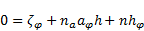
2. Preface to derivations
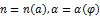
The region  (see Fig. 1) is the computation domain for the
solution to the Laplace’s differential equation that is going to be solved using the method of finite differences. The
inner border defined by the function
(see Fig. 1) is the computation domain for the
solution to the Laplace’s differential equation that is going to be solved using the method of finite differences. The
inner border defined by the function  is the contour of the
solenoid valve armature where:
is the contour of the
solenoid valve armature where:  . The outer border
given by the function
. The outer border
given by the function  is the inner side of
the magnet yoke. It should be noticed that following transformations are valid
only for the case of no contact between the armature and the inner side of the
magnet yoke neither at
is the inner side of
the magnet yoke. It should be noticed that following transformations are valid
only for the case of no contact between the armature and the inner side of the
magnet yoke neither at  nor at any other circumferential position
  . The room between the
borders has the permittivity compared to the permittivity of a vacuum.
. The room between the
borders has the permittivity compared to the permittivity of a vacuum.
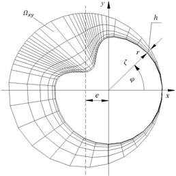
Fig. 1. Computation room
of the Laplace’s differential equation
The room is supposed to be
discretized in a particular manner. Mesh lines in a radial direction are
distorted in such a way that they exactly fit the inner and outer border. The
number of mesh lines in a radial direction is kept constant independently from
the distance  between the borders.
That means that at the circumferential position
between the borders.
That means that at the circumferential position  there is still a positive distance
  . In order to
visualise the capacity of the transformation this distance at was purposely set
in Figure 1 to a very small value. In general there is:
. In order to
visualise the capacity of the transformation this distance at was purposely set
in Figure 1 to a very small value. In general there is: 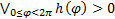 . This discretizing
method has the advantage that regions with small (in which the solution contributes dominantly to the sought force)
are meshed more densely than regions with big . That means that - in the difference to equidistant meshing methods
- one can avoid an unnecessary fine mesh in the case of big nonmagnetic gaps.
The density of mesh lines is variable both in the radial and peripheral
direction. This method of discretizing allows for increase of computation precision
with
a simultaneous reduction of the mesh node numbers.
. This discretizing
method has the advantage that regions with small (in which the solution contributes dominantly to the sought force)
are meshed more densely than regions with big . That means that - in the difference to equidistant meshing methods
- one can avoid an unnecessary fine mesh in the case of big nonmagnetic gaps.
The density of mesh lines is variable both in the radial and peripheral
direction. This method of discretizing allows for increase of computation precision
with
a simultaneous reduction of the mesh node numbers.
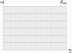
Fig. 2. Computation room of the Laplace’s differential equation
in  co-ordinate system
The aim of the work is to re-derive the
Laplace operator to a co-ordinates
system in which the computation domain gets a rectangle  shown in Figure 2. The derivation of the Laplace operator in
  co-ordinate system was done using the
following transformation:
co-ordinate system was done using the
following transformation:
 | (1) |
 | (2) |
Functions and  in (1) are restricted only to functions which
allow
in (1) are restricted only to functions which
allow  being isomorphic and
bijective in the whole domain . Furthermore, the range of
validity of the function is restricted to:
being isomorphic and
bijective in the whole domain . Furthermore, the range of
validity of the function is restricted to:  . In [1] this transformation was done using the transformation shoal
 | (3) |
with the operators:
 | (4) |
 | (5) |
 | (6) |
 | (7) |
The re-derivation of the Laplace operator will now be done in two
ways: using
the differential operators and using the differential geometry. In Table 1 the
overview of derivation ways is presented.
Table 1
Overview of derivation methods of Laplace
operator
|
Author
|
Vogel
|
Goraj
|
|
derivation using differential operators
|

|
|
|
derivation using the transformation shoal
|
|
not done
|
|
derivation using the differential geometry
|
not done
|
|
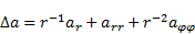
3. Derivation of Laplace operator
using differential operators
The Laplace operator in polar co-ordinate
system is given by [5]:
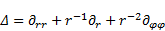 | (8) |
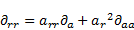
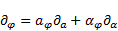
The differential operator  can be split using
rules of partial differentiation:
can be split using
rules of partial differentiation:
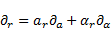 | (9) |
For the differential operator  can be written:
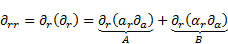 | (10) |
The application of the product rules on the term
A yields:
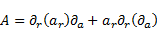 | (11) |
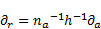
For the partial differential operator  can be written with
the use of (9)
can be written with
the use of (9)
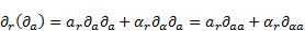 | (12) |
With the use of (12) the formula (11) can be simplified to:
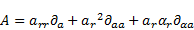 | (13) |
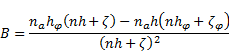
Analogously to A hold for B:
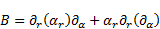 | (14) |
For the partial differential operator  one can use (9) again, which gives:
 | (15) |
The use of (15) in (14) yields:
 | (16) |
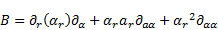
The summation of A and B yields
the operator
 | (17) |
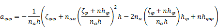
Analogously to (17), one obtains  :
:
 | (18) |
The unknowns in equations (17) and (18) are the first and the second derivative
of  and
and  in
in  and – direction. From the definition (2) one obtains:
 | (19) |
 | (20) |
The desolation of (1) for r leads to:
 | (21) |
The application of in (21) gives:
 | (22) |
The application of in (22) yields:
 | (23) |
The desolation of (22) for  and the desolation of (23) for
  results in:
 | (24) |
 | (25) |
The application of  in (21) yields:
 | (26) |
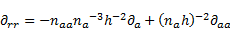
The application of in (26) yields:
 | (27) |
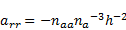
The desolation of (26) for  and the desolation of (27) for
  results in:
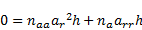
Setting of (28)
in (29) yields:
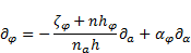
Setting of (9) and (17) in (19) and (20) yields:
 | (31) |
 | (32) |
After the replacement of and from (24) and (25) in (31) and (32), one
obtains the transformed differential operators and :
 | (33) |
 | (34) |
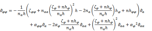
Setting now the relations (28) and (30) in (18) one gets the transformed differential
operator :
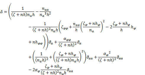
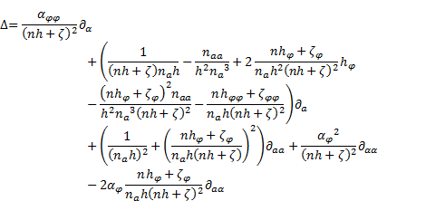
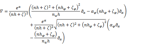
After setting of the operators (33) to (35) in (8) one obtains - under the usage of (1) - the Laplace operator in co-ordinate system:
The operator (36) is identical to the one derived in [1].
4. Derivation of Laplace operator using differential geometry
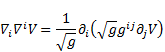
In differential geometry, the Laplace
operator can be generalized to operate on functions defined on surfaces in
Euclidean space. The more general operator is called the Laplace-Beltrami
operator. This operator of a scalar function in any
curvilinear co-ordinate system can be expressed using
Einstein notation [6-8]:
 in (37) is here the
contravariant metric tensor of the second rank. Its general covariant form is
[8]:
in (37) is here the
contravariant metric tensor of the second rank. Its general covariant form is
[8]:
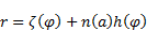
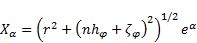
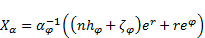
The  in (38) is the
summation index. The position vector
in (38) is the
summation index. The position vector  is defined by (39):
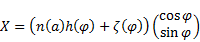 | (39) |
The variables of the position vector (39) are  and
and  . The derivatives
of the position vector (39) are:
. The derivatives
of the position vector (39) are:
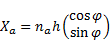 | (40) |
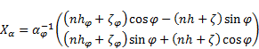 | (41) |
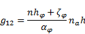
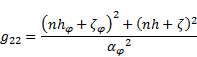
The use of (38) gives the components of the covariant metric tensors:
 | (42) |
 | (44) |
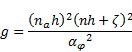
The determinant of the metric
tensors is equal to:
The contravariant metric tensor is defined as [6]:
 | (47) |
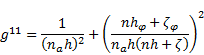
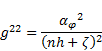
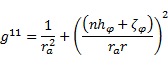
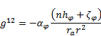
The components of the metric tensor in the
contravariant form are:
 | (50) |
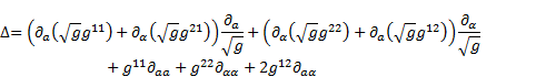
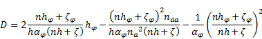
The Laplace operator simplifies in the
considered case to:
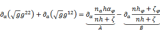
The multiplier of  can be expressed as:
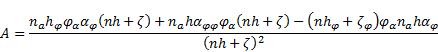
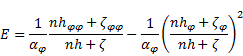
The first term of (53) is equal to:
The second term of (53) is equal to:
The subtraction of the terms (54) and (55) yields for (53):
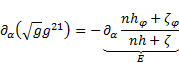
The first part-multiplier of  becomes:
The first term of (57) is equal to:
The second term of (57) is equal to:
The second part-multiplier of becomes:
Differentiation of (60) gives:
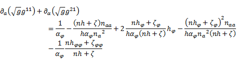
Addition of the terms  (58) and
  (59) together with
the subtraction of terms
(59) together with
the subtraction of terms  (61) results in the multiplier of . This multiplier equals:
Finally, inserting of (56), (62) and (46)-(51) in (52) yields to the Laplace operator:
The operator (63) is identical to (36) and to the one derived in [1].
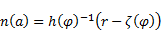
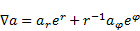
5. Gradient
The gradient of a scalar function  in any curvilinear co-ordinate system is
a covariant vector defined as [7]
in any curvilinear co-ordinate system is
a covariant vector defined as [7]
The derivatives of the position vector (39) are
given by (40) and (41). With the use of the new basis with unit
vectors:
 | (65) |
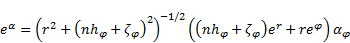 | (66) |
and the use of (1) one can write these derivatives in more
compact manner:
 | (67) |
 | (68) |
The gradient (64) can be expressed by its components as
follows:
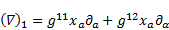 | (69) |
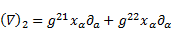 | (70) |
The elements of the contravariant metric tensor (48) to (51) can also be written in
a shorter way:
| (73) |
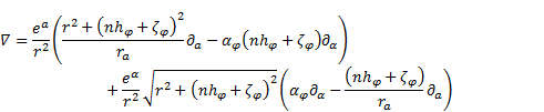
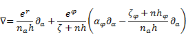
The sum of (69) and (70) together with (67), (68) and with relations (71)-(74) yields:
The derivatives of (1) in direction are:
 | (76) |
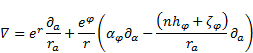
Setting of (1) and (76) in (75) results in the nabla operator in co-ordinate
system.
The operator (75) can also be expressed by means of the
unit vectors of the  basis:
Now the operator (78) can be inspected by means
of the operator (79) in polar
co-ordinate system [5]:
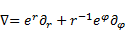 | (79) |
For the operator can be written by
means of rules of partial differentiation:
 | (80) |
Substitution of from (28) yields:
 | (81) |
After the setting of (19) and (24) in (9) one
obtains the operator :
 | (82) |
Finally, the usage of (81), (82) and (21) in (79)
yields to
 | (83) |
Under the use of (21), (76) one can see that the
operators (83) and (78) are identical to each other.
6. Vector surface element of the armature side surface
For the
parameterization of the armature side surface the position vector (39) must be extended in the axial
direction:
 | (84) |
The vector surface
element can be obtained from the cross product of partial
derivatives of (84) in the and  direction:
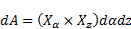 | (85) |
The derivatives of (84)
are:
 | (86) |
 | (87) |
Setting (86) and (87)
in (85) yields the vector surface element of the armature side surface
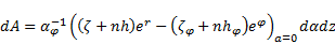 | (88) |
7. Conclusions
The Laplace
operator in the curvilinear co-ordinate system used for the numerical
computation of electromagnetic force acting on the armature of high-speed
solenoid valves was derived in three different ways: transformation shoal in [1], differential operators and differential
geometry. All these three Laplace operators are identical to each other.
References
[1]
Vogel R., Numerische Berechnung der Ankerreibung
eines elektromagnetischen Schaltventils, Studienarbeit, Universität Dortmund,
Dortmund 2006.
[2]
Peng L., Liyun F., Qaisar H., De X., Xiuzhen M.,
Enzhe S., Research on key factors and their interaction effects of
electromagnetic force of high-speed solenoid valve, The Scientific World
Journal 2014, p. Article ID 567242.
[3]
Huber B., Ulbrich H., Modeling and experimental
validation of the solenoid valve of a common rail diesel injector, SAE
Technical Paper 2014, 2014-01-0195.
[4]
Shahroudi K., Peterson D., Belt D., Indirect
adaptive closed loop control of solenoid actuated
gas and liquid injection valves, SAE Technical Paper 2006, 2006-01-0007.
[5]
Bronstein I.N., Semendjajew K.A., Musiol G., Mühlig
H., Taschenbuch der Mathematik, Edition Harri Deutsch, Berlin 2000.
[6]
Epstein M., Differential Geometry, Basic Notions
and Physical Examples, International Publishing: Springer, 2014.
[7]
McInerney A., First Steps in Differential
Geometry, Riemannian, Contact, Symplectic, Springer, New York 2013.
[8]
Nguyen-Schäfer H., Schmidt J.-P., Tensor
Analysis and Elementary Differential Geometry
for Physicists and Engineers, Springer, Berlin-Heidelberg 2014.