Numerical modeling of transient flows in load pipes with complex geometry
Sami Ramoul
,Ali Fourar
,Fawaz Massouh
Journal of Applied Mathematics and Computational Mechanics |
 Download Full Text |
 View in HTML format |
 Export citation |
@article{Ramoul_2017,
   doi = {10.17512/jamcm.2017.4.07},
   url = {https://doi.org/10.17512/jamcm.2017.4.07},
   year = 2017,
   publisher = {The Publishing Office of Czestochowa University of Technology},
   volume = {16},
   number = {4},
   pages = {67--78},
   author = {Sami Ramoul and  Ali Fourar and  Fawaz Massouh},
   title = {Numerical modeling of transient flows in load pipes with complex geometry},
   journal = {Journal of Applied Mathematics and Computational Mechanics}
}
TY - JOUR DO - 10.17512/jamcm.2017.4.07 UR - https://doi.org/10.17512/jamcm.2017.4.07 TI - Numerical modeling of transient flows in load pipes with complex geometry T2 - Journal of Applied Mathematics and Computational Mechanics JA - J Appl Math Comput Mech AU - Ramoul, Sami AU - Fourar, Ali AU - Massouh, Fawaz PY - 2017 PB - The Publishing Office of Czestochowa University of Technology SP - 67 EP - 78 IS - 4 VL - 16 SN - 2299-9965 SN - 2353-0588 ER -
Ramoul, S., Fourar, A., & Massouh, F. (2017). Numerical modeling of transient flows in load pipes with complex geometry. Journal of Applied Mathematics and Computational Mechanics, 16(4), 67-78. doi:10.17512/jamcm.2017.4.07
Ramoul, S., Fourar, A. & Massouh, F., 2017. Numerical modeling of transient flows in load pipes with complex geometry. Journal of Applied Mathematics and Computational Mechanics, 16(4), pp.67-78. Available at: https://doi.org/10.17512/jamcm.2017.4.07
[1]S. Ramoul, A. Fourar and F. Massouh, "Numerical modeling of transient flows in load pipes with complex geometry," Journal of Applied Mathematics and Computational Mechanics, vol. 16, no. 4, pp. 67-78, 2017.
Ramoul, Sami, Ali Fourar, and Fawaz Massouh. "Numerical modeling of transient flows in load pipes with complex geometry." Journal of Applied Mathematics and Computational Mechanics 16.4 (2017): 67-78. CrossRef. Web.
1. Ramoul S, Fourar A, Massouh F. Numerical modeling of transient flows in load pipes with complex geometry. Journal of Applied Mathematics and Computational Mechanics. The Publishing Office of Czestochowa University of Technology; 2017;16(4):67-78. Available from: https://doi.org/10.17512/jamcm.2017.4.07
Ramoul, Sami, Ali Fourar, and Fawaz Massouh. "Numerical modeling of transient flows in load pipes with complex geometry." Journal of Applied Mathematics and Computational Mechanics 16, no. 4 (2017): 67-78. doi:10.17512/jamcm.2017.4.07
NUMERICAL MODELING OF TRANSIENT FLOWS IN LOAD PIPES WITH COMPLEX GEOMETRY
Sami Ramoul 1, Ali Fourar 1, Fawaz Massouh 2
1
Faculty of Technology Hydraulics Department University of Batna2, Algeria
2 Laboratory of Fluid Mechanics at ENSAM, Paris, France
infodoc81@yahoo.com, fourarali05@hotmail.fr
Received: 7 October 2017;
Accepted: 23 December 2017
Abstract. Changes in the system flow of a fluid in a pipe often cause sudden pressure changes and give rise to so-called transient load flows. So, the study of the phenomenon of transient load flows aims to determine whether the pressure in the whole of a system is within the prescribed limits, following a perturbation of the flow. By defining the scope of a water hammer study, an examination is made of variations in velocity or flow and pressure resulting from poor operation of the hydraulic system, its normal operation and emergency operations. This paper introduces a numerical modeling of the phenomenon of transient flows in load pipes with variable geometries which presents a study of the average pressure and the average velocity of the transient flow in the pipe with quasi-steady term friction. The characteristic method is used to solve the governing equations of “Saint- -Venant”. Thanks to the AFT Impulse industrial program, we have obtained very interesting and very practical numerical results to describe the phenomenon of transient flows in variable load pipes.
MSC 2010: 35L02, 65M25
Keywords: numerical modeling, transient flow, water hammer, loaded pipes, characteristic method, AFT impulse software
1. Introduction
The transitional regime in hydraulic installations is a very complex phenomenon. It represents a permanent danger for installations and can occur at any time due to the various manipulations of the elements of the network.
The transient regime in the closed pipes is characterized by variations of the pressures, which are often very high or very low. These variations are accompanied by the phenomenon of propagation of the pressure waves that traverse the network for a certain time until their damping and the restoration of the initial regime [1]. This regime is the source of several damages (deterioration of the pipes) which incur often unforseen equipment and maintenance costs [2].
In this paper we will present a study of the average pressure and the average velocity of the transient flow in the pipe with quasi-steady term friction. Our objective in this contribution is to treat the most complex case, which means the theory of the hydraulic shock caused by the water hammer in the load pipes with variable geometry, going by way of the theoretical aspect; equations (mass conservation equation and momentum conservation equation).
From these equations, each method uses different simplifying hypotheses and/or resolving procedures, such as analytical, graphic or numerical methods [3]. But in view of the complexity of the phenomenon, there really are no complete analytical solutions to solve the problem, as in the case of Allievi’s method [4, 5], which gives us a global solution to the problem but does not take into account loss of loads which affects the extent of the phenomenon and the approximate graphic methods (such as the Schnyder-Bergeron method [6, 7]) that are not really effective in solving complex cases such as a pipe with several branches, or a pipe with variable characteristics, such as variations of the section, etc. So the numerical methods have taken over to allow us to quantify this type of phenomenon.
The objectives of this paper are on the one hand to study the causes of wave propagation, meaning a sudden stop of the water supply of the gravity loaded pipes. On the other hand we tried to formulate these phenomena as equations by taking essentials points the variations of the sections of the pipe and the closing of the valves. Rather we used the numerical method of the characteristics to solve the systems of equations representing transient flow. As tools of simulation we used AFT impulse software.
2. Basic assumptions and equations
2.1. Assumptions
The assumptions in the development of water hammer equations are [8]:
– flow in the pipeline is considered to be one - dimensional with the average velocity and the average pressure assumed to be uniform at a chosen section,
– the pipe is full and remains full during the transient,
– there is no column separation during the transient i.e. pressure is greater than the liquid vapor pressure,
– the pipe wall and the liquid behave linearly elastically,
– unsteady friction losses are approximated as steady state losses.
2.2. Basic wave propagation equations in pipes
The equations allow us to study all the transient phenomena that we meet in monophasic flow under pressure established by Saint-Venant are [9]:
Continuity equation
Dynamic equation
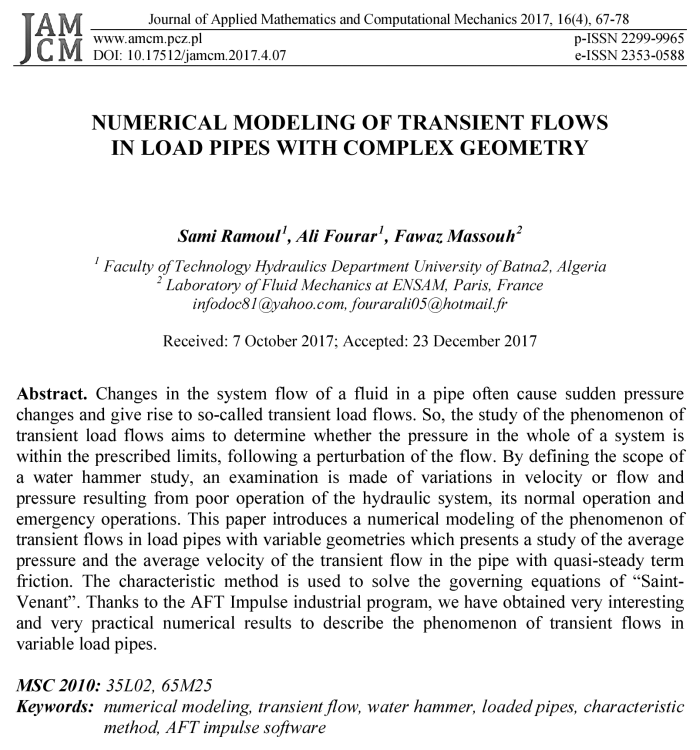
The friction factor f in equation (2) is expressed for the turbulent flow, from Colbrook formula (3)
 (3) (3) |
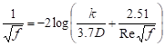
And the velocity of wave pressure is expressed by the relation (4)
 (4) (4) |
3. Method of characteristics
Based on the work of [10] and [11], we found that for a partial differential equation (PDE) of the first order, the characteristic method consists in searching for curves (called “characteristic lines” or simply “Characteristics”) along which the EDP is reduced to a simple ordinary differential equation (EDO). The resolution of the EDO along a characteristic makes it possible to find the solution of the original problem.
By multiplying equation (2) by an unknown constant λ, by adding it to equation (1), and rearranging and taking the total derivative, we obtain the following equations (5) and (7):
only when
While
only when
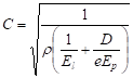
To understand the meaning of these four equations, it is necessary to examine them using the figure below (Fig. 1) [2].
Fig. 1. Characteristic lines
The resolution of equations (5) and (7) by the characteristic method consists in determining the head H and the average velocity U at the point P knowing the initial values at the points R and S. Let UP and HP be the parameters searched at point P. By multiplying equation (5) by dt and integrating, we obtain:
The term ![]() can
be evaluated as follows:
can
be evaluated as follows:
Assuming that velocity is constant at points R and P.
According to the degree of accuracy required, other approximations may be made, but they involve the unknown UP, hence the necessity of an iterative procedure to evaluate the term as well as possible.
Thus the equation becomes:
By the same approach, equation (7) can also be written:
In these relations, tp – 0 equal to Δt, and when these equations are multiplied by Δt they become:
| C+: |
And
| C–: |
Each of the characteristic equations can be integrated if:
4. Boundary conditions
The H and U values on the pipe ends are determined using boundary conditions. These conditions are:
4.1. Condition at the tank boundary
When the pipe outlet from a tank, the value of H remains constant for all times. In this case, it is assumed that:
This equation is solved simultaneously with the characteristic curve W–. We use equation (15) to obtain an expression for the velocity
4.2. Condition at the velocity boundary
If the velocity were known at the downstream end of a pipe, an expression of H is easily found. For example, suppose a valve is closed in a way that caused the speed to decrease linearly from U0 to zero in T seconds. The Up equation would be:
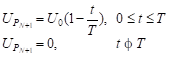 (19) (19) |
The equation for HP would be deduced from equation (14)
For any value of UPN+1 including zero.
5. Digital Data and results
5.1. Study model
In our work, we will base the comparison on the study models depicted by Figures 2 and 3. Rather Table 1 presents the parameters of the pipes and the fluid of our models.
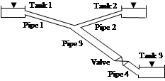
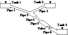
Fig. 2. Model 1, pipe of constant diameter Fig. 3. Model 2, pipe of variable diameter
Table 1
Parameters of the pipes and the fluid
|
Steel pipe |
L [m] |
D [mm] |
e [mm] |
k [mm] |
Ep [MPa] |
El [MPa] |
Tanks |
||
|
[H1] |
[H2] |
[H3] |
|||||||
|
Case 1 |
L1 |
400 |
202.71 |
3.22 |
0.0457 |
2·105 |
2053 |
161 |
161 |
20 |
|
L2 |
400 |
202.71 |
3.22 |
|||||||
|
L3 |
1990 |
202.71 |
3.22 |
|||||||
|
L4 |
100 |
202.71 |
3.22 |
|||||||
|
Case 2 |
L1 |
400 |
202.71 |
3.22 |
||||||
|
L2 |
400 |
202.71 |
3.22 |
|||||||
|
L3 |
800 |
202.71 |
3.22 |
|||||||
|
L4 |
400 |
154.05 |
2.80 |
|||||||
|
L5 |
790 |
202.71 |
3.22 |
|||||||
|
L6 |
100 |
202.71 |
3.22 |
|||||||
5.2. Slow closing
5.2.1. Case 1: slow closing of the valve with Constant diameter
|
|
|
|
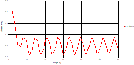
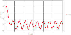
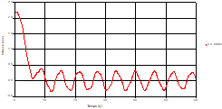
Fig. 4. Variation of head during time at the mid point of pipe 1 |
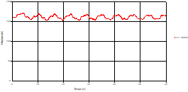
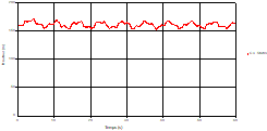
Fig. 5. Variation of velocity during time at the mid-point of the pipe 1 |
|
|
|
|
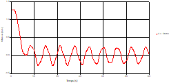
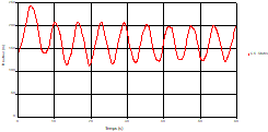
Fig. 6. Variation of head during time in pipe 3 at the point of intersection (connection) |
Fig. 7. Variation of velocity during time in pipe 3 at the point of intersection (connection) |
|
|
|
|
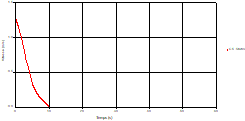
Fig. 8. Variation of head during time in pipe 3 at the mid-point |
Fig. 9. Variation of velocity during time in pipe 3 at the mid-point |
|
|
|
|
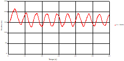
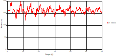
Fig. 10. Variation of head during time in pipe 3 to the valve |
Fig. 11. Variation of velocity during time in pipe 3 to the valve |
5.2.2. Case 2: slow closing of the valve with variable diameter
|
|
|
|
Fig. 12. Variation of height during time in pipe 1 at the mid-point |
Fig. 13. Variation of velocity during time in pipe 1 at the mid-point |
|
|
|
|
Fig. 14. Variation of head during time in pipe 3 at the point of intersection (connection) |
Fig. 15. Variation of velocity during time in pipe 3 at the point of intersection (connection) |
|
|
|
|
Fig. 16. Variation of head during time in pipe 4 at the mid-point |
Fig. 17. Variation of velocity during time in pipe 4 at the mid-point |
|
|
|
|
Fig. 18. Variation head during time in pipe 5 to the valve |
Fig. 19. Variation of velocity during time in pipe 5 to the valve |
5.2.3. Comparison of Case 1 and Case 2
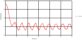
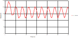
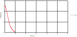
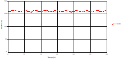
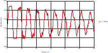
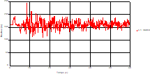
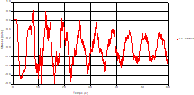
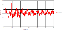
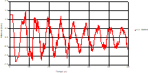
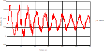
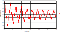
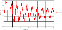
Based on the results presented by Figures 4 to 19, we found that at the two pipes C1 and C2: The amplitude of the variations in the piezometric head increases before closing the valve but with poor harmony, and it decreases until the closing of the valve to reach the initial values of the piezometric head in the case of rest but with very low oscillations. The attenuation of the fluctuations of the piezometric head is weak and slower each time we get closer to the tank, where the rate of fluctuations is almost identical in both cases. At C3 pipe at the branch: The amplitude of the variations in the piezometric head is greater than that of the first two pipes, and they remain in an oscillatory state with amplitudes more or less important until the end of the simulation. With regard to velocity; the value of the latter in the pipe C3 is twice that of the pipes C1 and C2, which explains the law of continuity. At pipe C4: The amplitude of the variations in the piezometric head is greater than that of the previous pipes. It is noted that the head losses are greater at the end of the pipe. At the valve: The amplitude of the fluctuations of the piezometric head increases at the midpoint and becomes maximum at the valve. The attenuations of the head fluctuations are less rapid at the mid-point and become increasingly slow every time one approaches the valve.
5.3. Rapid closing
5.3.1. Case 3: rapid closing with Constant diameter
|
|
|
|
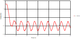
Fig. 20. Variation of head during time at the mid point of pipe 1 |
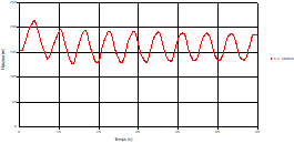
Fig. 21. Variation of velocity during time at the mid-point of the pipe 1 |
|
|
|
|
Fig. 22. Variation of head during time in pipe 3 at the point of intersection (connection) |
Fig. 23. Variation of velocity during time in pipe 3 at the point of intersection (connection) |
|
|
|
|
Fig. 24. Variation of head during time in pipe 3 at mid-point |
Fig. 25. Variation of velocity during time in pipe 3 at the mid-point |
|
|
|
|
Fig. 26. Variation of head during time in pipe 3 to the valve |
Fig. 27. Variation of velocity during time in pipe 3 to the valve |

5.3.2. Case 4: rapid closing with variable diameter
|
|
|
|
Fig. 28. Variation of head during time in pipe 1 at the midpoint |
Fig. 29. Variation of velocity during time in pipe 1 at the mid-point |
|
|
|
|
Fig. 30. Variation of head during time in pipe 3 at the point of intersection (connection) |
Fig. 31. Variation of velocity during time in pipe 3 at the point of intersection (connection) |
|
|
|
|
Fig. 32. Variation of head during time in pipe 4 at the mid-point |
Fig. 33. Variation of velocity during time in pipe 4 at the mid-point |
|
|
|
|
Fig. 34. Variation of head during time in pipe 5 to the valve |
Fig. 35. Variation of velocity during time in pipe 5 to the valve |
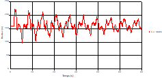
5.3.3. Comparison of Case 3 and Case 4
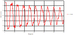
Based on the results presented by Figures 20 to 35, we found that at the C1 and C2 pipes: the amplitudes of the fluctuations of the piezometric head are faster and more pronounced in the point of intersection (connection) with maximum values at the beginning of the simulation and decreasing progressively over time. The attenuation of the fluctuations of the piezometric head is faster every time that one moves away from the tank, where the rate of fluctuations is almost identical in both cases.
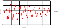
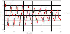
At the level of the pipe C3 connection: It is noted that the fluctuations of the head are very accentuated with oscillations greater than the two pipes and which decrease more in time. With regard to velocity; its value in pipe C3 is twice greater that of pipes C1 and C2, which explains the law of continuity. At pipe C4: The amplitude of the variations of the piezometric head is greater at the mid-point and becomes maximum at the change of section, and it remains in an oscillatory state with amplitudes more or less important until the end of the simulation. It will be noted that the velocity value in pipe C4 is very important as that of pipe C3. At the valve: The amplitude of the variations in the piezometric head is greater in case 4 at the midpoint than it is in case3 where the pipe is constant and becomes maximum at the valve. With regard to velocity; the amplitude of the variations in velocity decreases from the tank to the valve. The velocity fluctuations remain in an oscillatory state with more or less significant amplitudes until the end of the simulation. Velocity fluctuations are more pronounced at the level of the rapid closure.
6. Conclusions
We have proved in this paper that water hammer is a phenomenon that causes very detrimental effects on hydraulic pipes, such as fatigue, implosion and even breakage. It is especially true in the case of pipes with variable characteristics.
It is for this reason that our study, which takes into account the variations of the sections, has been directly concerned with the effect of the change of section on the evaluation of the phenomenon of hydraulic shock. Here, we should note that we have presented a deep study of the average pressure and the average velocity of the transient flow in the pipe with quasi-steady term friction. We have also based our work on the hyperbolic basic equations established by Saint-Venant; in this case the continuity equation and the dynamic equation to evaluate these transient phenomena. Also we used the method of characteristics to solve the systems of equations representing transient flow, we based these solution on the simplifying hypotheses mentioned above. In this work, which aims to approach the problem numerically, we used the AFT Impulse industrial program for the simulation of transient phenomena in complex hydraulic plant models and loaded hydraulic systems. Graphical results obtained from the variation of the piezometric head and the flow velocity over time, results in the necessity to always increase the time of manipulation and operation of the valves in order to decrease the amplitude variations in the piezometric head and the flow velocity and to avoid the change of the sections of the pipes and especially to calculate them so that they are resistant to these phenomena of overpressure and depression and in particular they must be resistant to the pressure where the vacuum is sufficient to create the cavitation. Moreover, our study was based on the case of one-dimensional flow without taking into account external changes such as changes in water temperature, density, etc.
|
Notations |
g |
Gravity acceleration [ms–2] |
|
|
|
U |
Average velocity [ms–1] |
C |
Velocity of wave pressure [ms–1] |
|
|
H |
The piezometric head [m] |
f |
Factor of friction |
|
|
D |
Inner pipe diameter [m] |
x |
Linear dimension [m] |
|
|
T |
Time [s] |
ρ |
Fluid density [kg m–3] |
|
|
El |
Bulk modulus of the liquid [Pa] |
e |
Pipe-wall thickness [m] |
|
|
Ep |
Young’s modulus [Pa] |
µ |
Dynamic viscosity [kg m–1s–1] |
|
|
L |
Pipe length [m] |
k |
Roughness Coefficient |
|
References
[1] Salah B., Kettab A., Massouh F., Bangangoye B., Célérité de l’onde de coup de bélier dans les réseaux enterrés, revue la Houille Blanche 2001, 3/4.
[2] Elaoud S., Hadj-Taïeb E., Influence of pump starting times on transient flows in pipes, Nuclear Engineering and Design 2011, 241, 3624-3631.
[3] Blommaert G., Étude du comportement dynamique des turbines francis, contrôle actif de leur stabilité de fonctionnement, Ph.D. thesis, Polytechnical School Fédérale de Lausanne 2000.
[4] Allevi L., Theorie general du movement varie de l’eau dans les tuyaux de conduit, Revue of Mechanics, Paris, France 1904, 14, 10-22 and 230-259.
[5] Allevi L., Colpo d’ariete e la regolazione delle turbine, Electtrotecnica 1932, 19, 146.
[6] Bertgeron L., Etude des variations de regime dans les conduits d’eau, Solution graphique generale, General Revue of Hydraulic 1935, 1, 12-69.
[7] Bergeron L., Etude des coups de belier dans les conduites, nouvel exose’ de la methode grphique, Revue La Technique Moderne 1936, 28, 33-75.
[8] Simpson A.R., Wu Z.Y., Computer Modelling of Hydraulic Transient in Pipe Networks and Associated Design Criteria. MODSIM97, International Congress on Modelling and Simulation, Modelling and Simulation Society of Australia, Hobart, Tasmania, Australia, 1997.
[9] Vaillant Y., Simulation du comportement transitoire de turbine Kalpan, Travail pratique de Master EPFL, Lausanne 2005, 85.
[10] Abuaziah I., Oulhaj A., Sebari K., Abbassi Saber A., Ouazar D., Shakameh N., Modeling and Controlling Flow Transient in Pipeline Systems, Rev. Mar. Sci. Agron. Vét. 2013, 3, 12-18.
[11] Siamao M., Mechanical interaction in pressurized pipe systems: experiments and numerical models, Journal of Water, Miklas scholz 2015, 7, 63261-6350.