Numerical calculations of the potential on the rectangular and ellpitic domains with various aspect ratios
Saeid Panahi
,Hassan Ghassemi
,Hashem Nowruzi
Journal of Applied Mathematics and Computational Mechanics |
 Download Full Text |
NUMERICAL CALCULATIONS OF THE POTENTIAL ON THE RECTANGULAR AND ELLPITIC DOMAINS WITH VARIOUS ASPECT RATIOS
Saeid Panahi, Hassan Ghassemi, Hashem Nowruzi
Department of Maritime Engineering, Amirkabir
University of Technology
Tehran, Iran
saeedpanahi@aut.ac.ir, gasemi@aut.ac.ir, h.nowruzi@aut.ac.ir
Received: 3 July 2017; Accepted: 11 September 2017
Abstract. In the current study, the Laplace equation is solved for rectangular and elliptical computational domains by using the boundary element method (BEM). For this accomplishment, 120 different aspect ratios in a rectangular and elliptical computational domains are designed. The Dirichlet and Neumann boundary conditions are used respectively for a rectangular and elliptical domains. Also, the Gaussian quadrature integral method is applied to solve the influence coefficient matrix in BEM. To assess a different aspect ratio on the potential solution, two different measurement positions are intended. According to our finding, with an increase of the aspect ratio, the potential value is increased for both rectangular and elliptical domains. However, a potential increment with aspect ratio enhancement is more visible in the elliptical domain.
MSC 2010:76M15, 76B07
Keywords: boundary element method, rectangular and elliptic domains, potential value
1. Introduction
Partial differential equations (PDEs) govern many engineering problems. In this regard, Laplace's equation is the simplest form of elliptic PDEs. Due to the simplicity and appropriate accuracy of Laplace's equation, it is used in different physical and engineering problems such as fluid dynamic [1], elasto-static [2], controls and vibrations [3] and heat transfer [4]. Potential theory is the general theory to solve Laplace's equation. Moreover, solutions of Laplace's equation are harmonic functions.
Much research is addressed towards a different method for solving Laplace’s equation under various boundary conditions [5-8]. For example, Laplace’s equation can be solved by separation of variables methods [9]. In the current study, we used this boundary element method (BEM) in solving Laplace’s equation. Several studies use the BEM to solve Laplace’s equation in different geometries and under different boundary conditions. For example, Mukherjee et al. [10] used the boundary node method for solving Laplace’s equation in the 2D domain. They studied the effect of different boundary conditions of Dirichlet, Neumann and mixed boundary conditions on the solution. Qian et al. [11] numerically solved Laplace’s equation in a rectangle by using the Cauchy problem method. They proposed two different regularization methods on the ill-posed problem based on separation of variables. Lesnic et al. [12] is also an iterative boundary element method to solve the Cauchy problem for Laplace’s equation. In another study, a semi-analytical method for solving Laplace’s equation with circular boundaries is proposed by Chen and Shen [13]. In their work, to avoid principal values of calculating, degenerate kernels are used. In addition, well-posed linear algebraic system, principal value free, elimi- nation of boundary-layer effect, exponential convergence and mesh free are advantages of their method. In other words, they have dealt with the singular integrals free of principal value sense due the utilization of degenerate kernel and their null-field integral approach. In another study, Chen et al. [14] focused on the connection between conformal mapping and curvilinear coordinates. They figured out the relation to take integration by way of mapping in the complex plane. In addition, solving Laplace’s problems by the image method in a spherical and circular domains are presented in Ref. [15] and [16], respectively.
Morales et al. [17] numerically studied the solutions of Laplace’s equation with simple boundary conditions. Their work was related to capacitors with multiple symmetries.
Analytical evaluation of the BEM singular integrals for 3D Laplace and Stokes flow equations using coordinate transformation is presented by Ren and Chan [18]. In their study, by applying a coordinate transformation, the analytical formulas of the singular integrals for 3D Laplace and Stokes flow equations are obtained for an arbitrary triangular boundary element with constant elements approximation. Jones and Moore [19] employed numerical technique to determine aerodynamic forces acting on oscillating surfaces in subsonic flow. Also, elementary calculations for three dimensional wings in steady flow have been presented. Sygulski [20] focused on vibrations of open membrane structures including interaction with air. Both FEM and BEM were used for the structure and the air respectively. The aerodynamic pressure and structure deformations are defined by boundary integral equations. In this paper, particular methods are applied to solve singular and non-singular integrals over whole domain. Cheng et al. [21] in a paper titled as “A fast adaptive multipole algorithm in three dimensions” used new compression techniques and diagonal forms for translation operators to achieve high accuracy at a reasonable cost. Fairweather et al. [22] conducted a numerical procedure to solve 2D potential problems using an improved boundary integral equation method. They used piecewise quadratic polynomial approximations in the boundary equation method for the solution of boundary value problems involving Laplace’s equation and certain Poisson equations. The boundary element method for the Dirichlet boundary condition of Laplace’s equation in elliptic domains with elliptic holes is used by Li et al. [23]. In this study, they developed the null field method for the elliptic domains with elliptic holes. Lee et al. [24] solved Laplace’s equation under Neumann condition in circular domains with circular holes by methods of field equations. Their results showed that MFEs is effective in solving Neumann problems. Recently, Yang [25] studied the Neumann problem of Laplace’s equation in semi convex domains.
On the other hand, the Robin problem for the Laplace’s equation in three dimensional star-like domains is investigated by Caratelli et al. [26]. They showed numerical procedure of relevant solutions derivation by using a suitable Fourier series-like method. Al-Khaled [27] focused on the numerical solutions of the Laplace equation. A reliable algorithm of the Adomian Decomposition Method (ADM) was employed to construct a numerical solution of Laplace’s equation. Dosiyev and Buranay [28] presented a one-block method to compute generalized stress intensity factors for Laplace’s equation on a square with a slit and on an L-shaped domains. Direct numerical identification of boundary values in the Laplace equation is investigated by Hayashi et al. [29]. Jorge et al. [30] focused on self-regular boundary integral equation formulations for Laplace’s equation in a 2D domain. In this work, application of the self-regular formulation strategy using Greens identity and its gradient form for Laplace’s equation is demonstrated. Chen [31] worked on a finite element model for solving Dirichlet’s problem of Laplace’s equation. His results are shown that this model is very efficient in obtaining the analytical solution over complex regions. Moreover, this method can be used to reduce main memory storage and computer time requirements.. Bamdadinejad et al. [32] studied on relative error changes of influence coefficients by using different Gaussian points to solve Laplace equation in rectangular domain. Ghassemi et al. [33] used a new numerical technique on discontinues boundary element method (DBEM) to solve Laplace equation. Finally, in our recent work, we solved Laplace’s equation by FDM and BEM using mixed boundary conditions [34].
According to cited works, lack of a comprehensive investigation on the solution of the Laplace equation for a rectangular and elliptical domains with a different aspect ratio and under different boundary conditions is evident. Therefore, in the present study, potential quantity in the rectangular and elliptical domains with different range of aspect ratio (a/b) (see Fig.1) is determined by solving the Laplace equation with BEM. In this study, we investigate the potential value on two different internal measurement nodes.
|
|
|
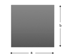
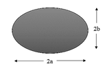
Fig. 1. Schematic of rectangular and elliptic domains and aspect ratio as (a/b)
The following sections are organized as follows. The computational procedure of BEM is reviewed in Section 2. In Section 3, the results of the potential on different internal measurement nodes of rectangular and elliptical domains with various aspect ratios are presented and discussed. Finally, Section 4 is given for the conclusions.
2. Computational procedure of BEM
The boundary element method (BEM) is an interesting method for solving partial differential equations (PDEs). The BEM is capable to apply for complex geometry with sharp changes. The reason behind this fact is related to limit all approximations in the BEM to the domain boundary. In this method, PDEs will be changed to integral equations forms which are applied on the surface or boundary of the considered domain. These integrals are numerically integrated over the boundary. Then, the boundary will be divided into small elements. Like other numerical methods, this procedure is continuing until a linear algebraic equation will be obtained which has only one answer. A schematic of the constant element is depicted in Figure 2. To describe of variable quantity and geometry form for each element, shape functions are used. These shape functions can be linear, quadratic and higher orders.
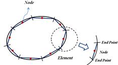
Fig. 2. Schematic of constant element
On the other hand, due to the complexity of integrating functions, analytical integration is not suitable to calculate the integrals. Therefore, the Gaussian square method is recommended. It’s also notable that the total integral will be formed by adding all the integrals of all elements.
In the BEM, the integral formulation for the domain and its boundary is presented in the following expression
| (1) |
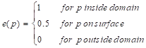
where p is
considered point and ![]() is
is
 | (2) |
Term of G in Eq. (1) is the Green’s function of the Laplace equation. Also, discretization of the Eq. (1) has the following form
| (3) |
| where |
| (4) |
where
n is the number of integration points (Gauss points) and ![]() is length of each element. In addition,
is length of each element. In addition, ![]() and
and ![]() are
the abscissas and weights of the Gaussian quadrature of order n, respectively.
Also, the integral of
are
the abscissas and weights of the Gaussian quadrature of order n, respectively.
Also, the integral of ![]() for off diagonal elements can
also be calculated analytically by
for off diagonal elements can
also be calculated analytically by
| (5) |
Now, to calculate the on-diagonal influence matrix, Eqs. (6) and (7) are governed
| (6) |
| (7) |
It should be noted that for higher order elements analytical integration is not |applicable, and for this reason, other integration techniques due to the type of singularity are employed [35].
For assessment of our numerical results from BEM, two different measurement positions as N and E are assumed. These considered measurement positions in rectangular and elliptical domains are depicted in Figure 3. The reason for this selection is due to symmetry of our domain for N internal node with S and E internal node with W.
|
|
|
|
(a) |
(b) |

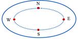
Fig. 3. Two considered measurement position as internal node in: a) rectangular and b) elliptical domain
3. Results and discussion
3.1. Aspect ratio vs. potential in rectangular domain
The potential value for two different internal nodes of N and E under a different aspect ratios in a rectangular domain from BEM is illustrated respectively in Figures 4 and 5. According to Figures 4 and 5, it is visible that by increasing the aspect ratio until about a/b = 100, potential value is increased with remarkable growth rate. For simplification, this conversion is more specified in a/b < 1. Also, small ascending tendency has shown between 1 and 100. However, for a/b > 100, the answer gradually converged at potential value of 50 and 75 for E and N nodes. The reason for this convergence is the summation form of the answer depended to sinus and hyperbolic sinus solution. In large aspect ratios, arguments of these trigonometric functions tend to a little value. Because of equivalence of sinus with Theta the answer equals to Theta.
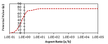
Fig. 4. Potential value from BEM in rectangular domain under different aspect ratios at measurement point of N
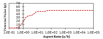
Fig. 5. Potential value from the BEM in rectangular domain under different aspect ratios at the measurement point of E
3.2. Aspect ratio vs. potential in elliptical domain
The potential value for two different internal nodes of N and E under a different aspect ratio in elliptical domain from the BEM is depicted respectively in Figures 6 and 7. Based on Figure 6, it is visible that by increasing the aspect ratio until 1E+2, approximately similar value for potential value is obtained. However, after this a/b, a jump in the potential value in the start of each interval of a/b is visible. The reason that this happens is due to a change in the number of elements in each aspect ratio intervals. Based on Figure 7, by increasing the aspect ratio until 1E-1, the increment of logarithmic potential value is visible. After this a/b, a similar value of the potential is increased but in more inclination than a/b < 0.1.
Fig. 6. Potential value from BEM in elliptical domain under different aspect ratios at measurement point of N
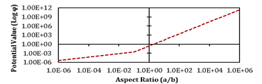
Fig. 7. Potential value from BEM in elliptical domain under different aspect ratios at measurement point of E
3.3. Potential distribution around the rectangular domain
Based on the boundary conditions of the rectangular domain, from the numerical solution of BEM, we can obtain the derivative of potential in each point on the boundary at first, and then solve this problem for every internal nodes we need. For this reason, we demonstrate the absolute potential derivative distribution on the boundary for specific aspect ratio 5/3 with 64 elements in Figure 8. Due to the shape of this distribution, the number of elements is not really effective as much as the elliptical domain. Also, because of a large range of potential derivative values for each side of this rectangle, scale factors are used to illustrate distribution clearly. Scale factors are 0.25, 0.01, 0.01 and 0.01 for bottom, right, top and left hand side of intended rectangle.
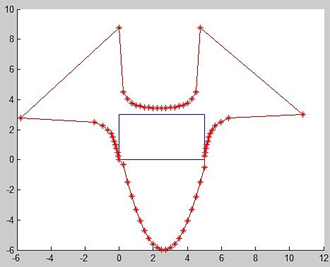
Fig. 8. Absolute potential derivative distribution around rectangular domain for a/b = 5/3 with 64 elements
3.4. Potential distribution around the elliptical domain
Potential distribution for two different numbers of elements, 20 and 64, under the Neumann boundary condition in elliptical domain from BEM is depicted respectively in Figure 9. In the elliptical domain due to boundary conditions, the potential values are unknown on each point of the boundary. It is visible that an increase in the number of elements results in a smoother potential value curve. So, based on Figures 9a and 9b, the effect of the number of elements in the potential value at each point of the boundary, for a specific aspect ratio of 5/3, is presented.
|
|
|
|
(a) |
(b) |
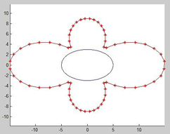
Fig. 9. Potential distribution around elliptical domain for a/b = 5/3 with (a) 20 elements and (b) 64 elements
4. Conclusions
The Laplace equation is specific and useful PDE which is governing in different physical and engineering problems. One the other hand, the boundary element method (BEM) is a reliable method in solving the Laplace equation. Therefore, in the current study, effects of different aspect ratio on potential value in rectangular and elliptic domainss are investigated by solving the Laplace equation using BEM. For this accomplishment, 120 different aspect ratios for rectangular and elliptical domains are considered. It’s notable that the Dirichlet and Neumann boundary conditions are used respectively in the rectangular and elliptical domains. In addition, the Gaussian quadrature method is used to calculate the influence coefficient matrices. Among the most important extracted findings in this study are the following:
1. By increasing the aspect ratio in the rectangular and elliptical domains, the potential value is increased for each measurement position.
2. Approximately, the parabolic trend is visible with an aspect ratio increment for both computational domains.
3. By increment 1E+5 times in aspect ratio of rectangular domain, 11% and 2.073% growth is detected for potential value in E and N nodes. In addition, with increment 1E+5 times in aspect ratio of elliptical domain, 1.009 E12 % and 1736.36% growth is obtained for potential value in E and N nodes, respectively.
References
[1] Blazek J., Computational fluid dynamics: principles and applications, Butterworth-Heinemann, 2015.
[2] Wang H., Yao Zh., Application of a new fast multipole BEM for simulation of 2D elastic solid with large number of inclusions, Acta Mechanica Sinica 2004, 6, 613-622.
[3] Li G., Xing-Yuan M., Yuan-Tai H., Wang J., Analysis of smart beams with piezoelectric elements using impedance matrix and inverse Laplace transform, Smart Materials and Structures 2013, 22, 11, 115001.
[4] Tarasov V.E., Heat transfer in fractal materials, International Journal of Heat and Mass Transfer 2016, 93, 427-430.
[5] Smith G.D., Numerical Solution of Partial Differential Equations: Finite Difference Methods, Oxford University Press, 1985.
[6] Chen J.T., Lin S.R., Chen K.H., Degenerate scale problem when solving Laplace's equation by BEM and its treatment, International Journal for Numerical Methods in Engineering 2005, 62, 233-261.
[7] Peaceman D.W., Henry H., Rachford, Jr., The numerical solution of parabolic and elliptic differential equations, Journal of the Society for Industrial and Applied Mathematics 1955, 3, 28-41.
[8] Gerdes K., Demkowicz L., Solution of 3D-Laplace and Helmholtz equations in exterior domains using hp-infinite elements, Computer Methods in Applied Mechanics and Engineering 1996, 137, 3-4, November.
[9] Kalnins E., On the separation of variables for the laplace equation Δψ+K^2ψ=0 in two-and three-dimensional Minkowski space, SIAM Journal on Mathematical Analysis 1975, 6, 340-374.
[10] Mukherjee Y.X., Subrata M., The boundary node method for potential problems, International Journal for Numerical Methods in Engineering 1997, 40, March, 797-815.
[11] Zhi Qian, Chu-Li Fu, Zhen-Ping Li, Two regularization methods for a Cauchy problem for the Laplace equation, Journal of Mathematical Analysis and Applications 2008, 338, 479-489.
[12] Lesnic D., Elliott L., Ingham D.B, An iterative boundary element method for solving numerically the Cauchy problem for the Laplace equation, Engineering Analysis with Boundary Elements 1997, 20, 2, September.
[13] Jeng-Tzong Chen, Wen-Cheng Shen, Null-field approach for Laplace problems with circular boundaries using degenerate kernels, Numerical Methods for Partial Differential Equations 2009, 25, 63-85.
[14] Jeng-Tzong Chen, Ming-Hong Tsai, Chein-Shan Liu, Conformal mapping and bipolar coordinate for eccentric Laplace problems, Computer Applications in Engineering Education 2009, 18, September.
[15] Chen J.T., Shieh H.C., Lee Y.T., Lee J.W., Bipolar coordinates image method and the method of fundamental solutions for Green’s functions of Laplace problems containing circular boundaries. 2011, Vol. 35, 236-243.
[16] Chen J.T., Shieh H.C., Lee Y.T., Lee J.W., Image solutions for boundary value problems without sources, Applied Mathematics and Computation 2010, 216, May.
[17] Morales M., Rodolfo Diaz R.A., Herrera W.J., Solutions of Laplace’s equation with simple boundary conditions, and their applications for capacitors with multiple symmetries, Journal of Electrostatics 2015, 78, 31-45.
[18] Qinlong Ren, Cho Lik Chan, Analytical evaluation of the BEM singular integrals for 3D Laplace and Stokes flow equations using coordinate transformation, Engineering Analysis with Boundary Elements 2015, 53, 1-8.
[19] Jones W.P., Moore J.A., Simplified aerodynamic theory of oscillating thin surfaces in subsonic flow, American Institute of Aeronautics and Astronautics 1973, 11, 1305-1307.
[20] Sygulski R., Dynamics analysis of open membrane structures interacting with air, International Journal for Numerical Methods in Engineering 1994, 37, 1807-1823.
[21] Cheng H., Greengard L., Rokhlin V., A fast adaptive multipole algorithm in three dimensions, Journal of Computational Physics 1999, 155, 2, November.
[22] Graeme Fairweather, Frank J Rizzo, David J Shippy, Yensen S Wu, On the numerical solution of two-dimensional potential problems by an improved boundary integral equation method, Journal of Computational Physics 1979, 31, 1, April.
[23] Li Z.C., Zhang L.P., Wei Y., Lee M.G., Chiang J.Y., Boundary methods for Dirichlet problems of Laplace’s equation in elliptic domains with elliptic holes, Engineering Analysis with Boundary Elements 2015, 61, December.
[24] Lee M.G., Li Z.C., Huang H.T., Chiang J.Y., Neumann problems of Laplace’s equation in circular domains with circular holes by methods of field equations, Engineering Analysis with Boundary Elements 2015, 51, February.
[25] Sibei Yang, The Neumann problem of Laplace’s equation in semionvex domains, Nonlinear Analysis: Theory, Methods & Applications 2016, 133, March.
[26] Caratelli D., Ricci P.E., Gielis J., The Robin problem for the Laplace equation in a three dimensional star like domain, Applied Mathematics and Computations 2011, 218, 3, October.
[27] Kamel Al-Khaled, Numerical solutions of the Laplace’s equation, Applied Mathematics and Computations 2005, 170, 2, November.
[28] Dosiyev D.D., Buranay S.C., One-block method for computing the generalized stress intensity factors for Laplace’s equation on a square with a slit and on an L-shaped domain, Journal of Computational and Applied Mathematics 2015, 289, December.
[29] Keysuke Hayashi, Kazuei Onishi, Yoko Ohura, Direct numerical identification of boundary values in the Laplace equation, Journal of Computational and Applied Mathematics 2003, 152, March.
[30] Jorge A.B., Riberio G.O., Cruse T.A., Fisher T.S., Self-regular boundary integral equation formulations for Laplace’s equation in 2-D, International Journal for Numerical Methods in Engineering, 2001, March.
[31] Chen Y.H., On a finite element model for solving Dirichlet’s problem of Laplace’s equation, International Journal for Numerical Methods in Engineering 1982, May.
[32] Bamdadinejad M., Ghassemi H., Ketabdari M.J., Calculation of quantity rate on the rectangular domain by boundary element method, Applied Mathematics and Physics 2017, 5, 40-46.
[33] Ghassemi H., Ahani A., Solving the quantity element using new numerical techniques on the discontinues boundary element method, American Journal of Applied Mathematics and Statistics 2017, 5, 14-21.
[34] Ghassemi H., Panahi S., Kohnsal A.R., Solving the Laplace’s equation by FDM and BEM using mixed boundary conditions, American Journal of Applied Mathematics and Statistics 2016, 4, 37-42.
[35] Katsikadelis J.T., Boundary Element, Theory and Application, Elsevier Publication, 2002.