Some closed-form bending formulas for elastically restrained Euler-Bernoulli beams under point and uniformly distributed loads
Vebil Yıldırım
Journal of Applied Mathematics and Computational Mechanics |
 Download Full Text |
 View in HTML format |
 Export citation |
@article{Yıldırım_2018,
   doi = {10.17512/jamcm.2018.3.09},
   url = {https://doi.org/10.17512/jamcm.2018.3.09},
   year = 2018,
   publisher = {The Publishing Office of Czestochowa University of Technology},
   volume = {17},
   number = {3},
   pages = {97--109},
   author = {Vebil Yıldırım},
   title = {Some closed-form bending formulas for elastically restrained Euler-Bernoulli beams under point and uniformly distributed loads},
   journal = {Journal of Applied Mathematics and Computational Mechanics}
}
TY - JOUR DO - 10.17512/jamcm.2018.3.09 UR - https://doi.org/10.17512/jamcm.2018.3.09 TI - Some closed-form bending formulas for elastically restrained Euler-Bernoulli beams under point and uniformly distributed loads T2 - Journal of Applied Mathematics and Computational Mechanics JA - J Appl Math Comput Mech AU - Yıldırım, Vebil PY - 2018 PB - The Publishing Office of Czestochowa University of Technology SP - 97 EP - 109 IS - 3 VL - 17 SN - 2299-9965 SN - 2353-0588 ER -
Yıldırım, V. (2018). Some closed-form bending formulas for elastically restrained Euler-Bernoulli beams under point and uniformly distributed loads. Journal of Applied Mathematics and Computational Mechanics, 17(3), 97-109. doi:10.17512/jamcm.2018.3.09
Yıldırım, V., 2018. Some closed-form bending formulas for elastically restrained Euler-Bernoulli beams under point and uniformly distributed loads. Journal of Applied Mathematics and Computational Mechanics, 17(3), pp.97-109. Available at: https://doi.org/10.17512/jamcm.2018.3.09
[1]V. Yıldırım, "Some closed-form bending formulas for elastically restrained Euler-Bernoulli beams under point and uniformly distributed loads," Journal of Applied Mathematics and Computational Mechanics, vol. 17, no. 3, pp. 97-109, 2018.
Yıldırım, Vebil. "Some closed-form bending formulas for elastically restrained Euler-Bernoulli beams under point and uniformly distributed loads." Journal of Applied Mathematics and Computational Mechanics 17.3 (2018): 97-109. CrossRef. Web.
1. Yıldırım V. Some closed-form bending formulas for elastically restrained Euler-Bernoulli beams under point and uniformly distributed loads. Journal of Applied Mathematics and Computational Mechanics. The Publishing Office of Czestochowa University of Technology; 2018;17(3):97-109. Available from: https://doi.org/10.17512/jamcm.2018.3.09
Yıldırım, Vebil. "Some closed-form bending formulas for elastically restrained Euler-Bernoulli beams under point and uniformly distributed loads." Journal of Applied Mathematics and Computational Mechanics 17, no. 3 (2018): 97-109. doi:10.17512/jamcm.2018.3.09
SOME CLOSED-FORM BENDING FORMULAS FOR ELASTICALLY RESTRAINED EULER-BERNOULLI BEAMS UNDER POINT AND UNIFORMLY DISTRIBUTED LOADS
Vebil Yıldırım
Department of Mechanical Engineering,
University of Çukurova
Adana, Turkey
vebil@cu.edu.tr
Received: 19 July 2018;
Accepted: 28 October 2018
Abstract. The transfer matrix method based on the Euler-Bernoulli beam theory is employed in order to originally achieve some exact analytical formulas for elastically supported beams under a point force together with uniformly distributed force and uniformly distributed couple moments. Those closed-form formulas can be used in a variety of engineering applications especially at the pre-design stage to get an insight into the response of the structure. Contrary to the classical boundary conditions, it is also observed that the Euler-Bernoulli solutions of a beam with elastic supports are sensitive to the ratio of length to thickness (L/h).
MSC 2010: 74K10, 74B05, 35C05, 35G10
Keywords: Euler-Bernoulli beam, elastic support, transfer matrix method, initial value problem, bending
1. Introduction
As it is well known, the Euler-Bernoulli beam theory (also known as the engineer’s beam theory or classical beam theory), which was first introduced circa 1750, still provides a simple calculation tool to analyse numerous static and dynamic engineer- ing problems [1-5]. The underlying well-known assumptions in the Euler-Bernoulli theory are: i) The cross-section is infinitely rigid in its own plane, ii) The cross-section of a beam remains plane after deformation, iii) The plane section initially perpendicular to the mid-surface will remain normal to the deformed axis of the beam. Based on the experimental measurements, these assumptions are held for long and slender beams.
The transfer matrix method also provides the scientists with a simple tool to model and solve one-dimensional problems [6-9]. The simplicity and easy programmability of the transfer matrix method makes it an alternative method to the finite elements in structural and mechanical engineering.
The present study is a continuation of Ref. [9] in which some exact analytical bending formulas for classically supported Euler-Bernoulli beams under both concentrated and generalized power/sinusoidal distributed loads were offered. As stated in the Abstract, an Euler-Bernoulli beam supported by both linear and rotational springs is to be considered in the present bending analysis.
2. Application of the Transfer Matrix Method
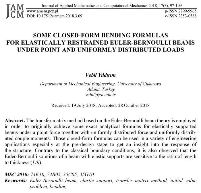
Let x be the beam axis, and let’s use the prime symbol for the derivative of the related quantity with respect to x. The governing homogeneous differential equation set for the out-of-plane bending analysis of the beam having a uniform section in canonical form is given by [6]
|
|
 ,
, 
where ![]() is called the state
vector which comprises the cross-sectional quantities at a positive section,
is called the state
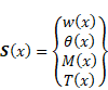
vector which comprises the cross-sectional quantities at a positive section, ![]() is the differential
matrix,
is the differential
matrix, ![]() is the transverse displacement
along z-axis,
is the transverse displacement
along z-axis, ![]() is the rotation about y-axis,
is the rotation about y-axis,
![]() is the bending moment,
and
is the bending moment,
and ![]() is the shear force,
and
is the shear force,
and ![]() is the bending
rigidity. Let’s denote the unit matrix by
is the bending
rigidity. Let’s denote the unit matrix by ![]() to determine
the characteristic equation of the differential matrix
as follows
to determine
the characteristic equation of the differential matrix
as follows
|
|
Since every square matrix satisfies its own
characteristic equation according to the Cayley-Hamilton theorem, ![]() is held. This means
that the higher powers of the differential matrix that are equal or greater
than four are identically zero.
is held. This means
that the higher powers of the differential matrix that are equal or greater
than four are identically zero.
Both the state vector and the transfer matrix satisfy the similar type of differential equation as in Eq. (1) [6]:
|
|
|
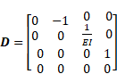
If the elements of ![]() are constants
as in Eq. (1), one may get an exact transfer matrix.
In this case, the solution of Eq. (3) with the initial conditions,
are constants
as in Eq. (1), one may get an exact transfer matrix.
In this case, the solution of Eq. (3) with the initial conditions, ![]() ,
gives
,
gives ![]() as follows:
as follows:
|
|
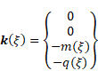
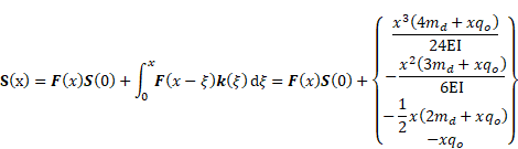
Let’s assume that the beam is to be subjected
to both a distributed force ![]() and a distributed
couple moment m
and a distributed
couple moment m![]() along the beam axis
together with a concentrated force
along the beam axis
together with a concentrated force ![]() and a couple moment
and a couple moment ![]() acting at section
acting at section ![]() . Under this
assumption, the overall transfer matrix relates the state vectors at both ends
of the beam
as follows:
. Under this
assumption, the overall transfer matrix relates the state vectors at both ends
of the beam
as follows:
|
|
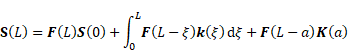
where ![]() stands for the
nonhomogeneous solution due to the distributed forces, and
stands for the
nonhomogeneous solution due to the distributed forces, and ![]() is referred to as a
discontinuity matrix due to the intermediate point loads
is referred to as a
discontinuity matrix due to the intermediate point loads
|
|
 ,
, 
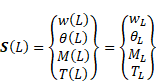
For short, let’s use the following for symbolizing the elements of the state vectors at two ends
|
|
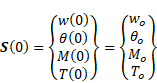 ,
, 
Boundary conditions considered in the present
study are shown in Figure 1 and Table 1. In Figure 1 and Table 1, ![]() and
and ![]() stand for the linear
spring constants at the initial and final ends, respectively. The rotational
spring constants at the ends are represented by
stand for the linear
spring constants at the initial and final ends, respectively. The rotational
spring constants at the ends are represented by ![]() and
and ![]() .
.
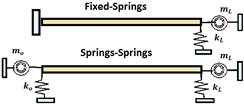
Fig. 1. Elastically supported beams
Table 1
Boundary conditions considered
|
|
|
|
|
Clamped-Elastic (C-E) |
|
|
|
Elastic-Elastic (E-E) |
|
|
In the transfer
matrix method, after evaluation of the transfer matrix, it is essential to
calculate whole elements the whole elements of the initial state vector as
a second key stage of the procedure. To do this, the boundary conditions given
at both ends (Table 1) should be implemented into Eq. (5) to form the equations
for the unknown quantities at the initial end of the beam. The unknown elements
of the initial state vector are then obtained from the solution of the equations
generated
in this way. After determination of the full elements of ![]() , all sectional
quantities at any section may be computed in a straight way as follows
, all sectional
quantities at any section may be computed in a straight way as follows
|
|
In the following two sections, the analytical formulas are to be derived for beams under separate distributed and concentrated loads. Since small deformations are assumed, the superposition principle is held when necessary.
3. Solutions for uniformly distributed forces
If only uniformly
distributed forces and couple moments are concerned, ![]() and
and ![]() , a general solution
takes the following form
, a general solution
takes the following form ![]()
|
|
3.1. A C-E beam under uniformly distributed loads
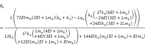
In a C-E beam, the unknown elements of the initial state vector are found as follows after implementation of the boundary conditions as (Table 1)
|
|
|
|
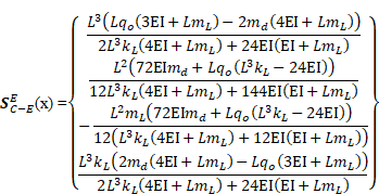
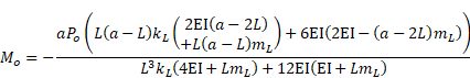
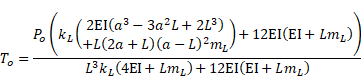
Cross-sectional quantities are then derived in closed forms as
|
|
Dimensionless transverse displacements under
uniform loads are defined as
![]() . As a numerical
example, two different spring constants
are studied. They are chosen as
. As a numerical
example, two different spring constants
are studied. They are chosen as ![]() and
and ![]()
![]() . The properties of the beam with a square
section are:
. The properties of the beam with a square
section are: ![]() .
Dimensionless transverse displacements in a C-E beam based on the two beam
theories are shown in Figure 2 and Table 2. For
.
Dimensionless transverse displacements in a C-E beam based on the two beam
theories are shown in Figure 2 and Table 2. For ![]() , the Timoshenko
solution gives higher transverse dimensionless displacements for all soft and
stiff elastic springs.
, the Timoshenko
solution gives higher transverse dimensionless displacements for all soft and
stiff elastic springs.
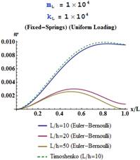
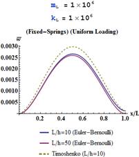
Fig. 2. Dimensionless transverse displacements in a C-E beam based on the two beam theories
Table 2
Transverse displacements in C-E and E-E beams under uniformly distributed forces
|
x/L |
L/h = 10 |
L/h = 20 |
L/h = 50 |
L/h = 10 |
L/h = 20 |
|
|
|||||
|
C-E Timoshenko |
E-E Timoshenko |
||||
|
0. |
0. |
0. |
0. |
0.000125 |
7.8125.10–6 |
|
0.2 |
0.00128868 |
0.00111953 |
0.00107501 |
0.001403 |
0.00112669 |
|
0.6 |
0.00279552 |
0.00248325 |
0.00241261 |
0.002842 |
0.00248612 |
|
1. |
0.000124607 |
7.81093.10–6 |
1.99999.10–7 |
0.000125 |
7.8125.10–6 |
|
|
C-E Euler-Bernoulli |
E-E Euler-Bernoulli |
|||
|
0. |
0. |
0. |
0. |
0.000125 |
7.8125.10–6 |
|
0.2 |
0.00108028 |
0.00106752 |
0.00106669 |
0.001195 |
0.00107469 |
|
0.6 |
0.00248371 |
0.00240525 |
0.00240013 |
0.00253 |
0.00240812 |
|
1. |
0.000124595 |
7.81091.10–6 |
1.99999.10–7 |
0.000125 |
7.8125.10–6 |
|
|
|
||||
|
C-E Timoshenko |
E-E Timoshenko |
||||
|
0. |
0. |
0. |
0. |
0.0125 |
0.00078125 |
|
0.2 |
0.00232318 |
0.00120285 |
0.00107717 |
0.0140921 |
0.00192069 |
|
0.6 |
0.00901646 |
0.00299159 |
0.00242591 |
0.0156882 |
0.0032904 |
|
1. |
0.00961267 |
0.000765863 |
0.0000199896 |
0.0125 |
0.00078125 |
|
|
C-E Euler-Bernoulli |
E-E Euler-Bernoulli |
|||
|
0. |
0. |
0. |
0. |
0.0125 |
0.00078125 |
|
0.2 |
0.00207851 |
0.00115022 |
0.00106885 |
0.0138841 |
0.00186869 |
|
0.6 |
0.00867176 |
0.00291381 |
0.00241343 |
0.0153762 |
0.0032124 |
|
1. |
0.00954707 |
0.000765746 |
0.0000199896 |
0.0125 |
0.00078125 |
Contrary to the
classical supports, Euler-Bernoulli solutions of beams with
elastic supports display sensitivity to the ratio of ![]() . Develops with using
much softer springs (Consider revising here. Oddly-worded and not sure of
intent). Soft springs make the transverse dimensionless displacements higher at
the elastically supported ends. Those displacements decrease with increasing
ratios of
. Develops with using
much softer springs (Consider revising here. Oddly-worded and not sure of
intent). Soft springs make the transverse dimensionless displacements higher at
the elastically supported ends. Those displacements decrease with increasing
ratios of ![]() for
the same beam. As it is well known, when both spring constants get larger and
larger, viz., when
for
the same beam. As it is well known, when both spring constants get larger and
larger, viz., when ![]() and
and ![]() , the elastic supports
turn to be rigid ones
in the limit case.
, the elastic supports
turn to be rigid ones
in the limit case.
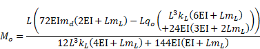
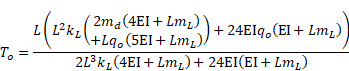
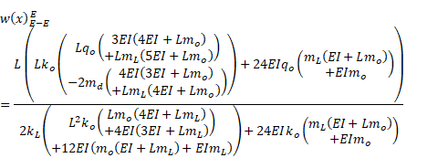
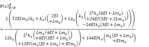
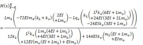
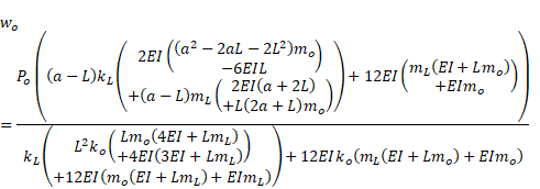
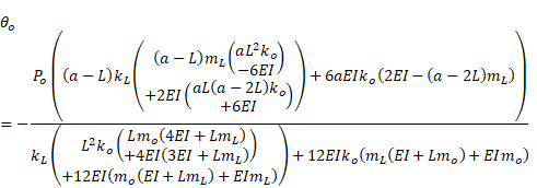
3.2. An E-E beam under uniformly distributed loads
The beam is, now,
assumed to be elastically supported at two ends by using both the linear and
rotational springs (Fig. 1). The elements of ![]() are as follows
are as follows
|
|
||||
|
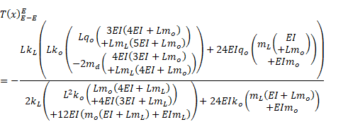
Sectional quantities along the beam are explicitly presented in Eq. (13):
|
|
||||
|
|
|
|
||||
|
|
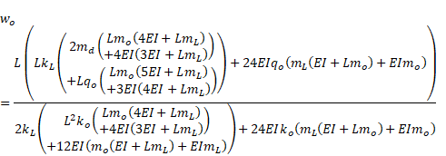
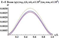
A variation of the
dimensionless transverse displacement in an E-E beam is demonstrated in Figure
3 for two different spring constants that have been studied in the previous
example. Some values of the transverse displacements in an E-E beam based on
the two beam theories are also given in Table 2. From Figure 3,
a symmetric variation of the transverse displacement is observed due to the
symmetric loads and geometry. It is observed from both Table 2 and Figure 3
that an increase in the spring constants
results in a decrease in the transverse displacements. In other words,
the softer the springs, the greater the dimensionless displacements at both
ends. The differences in the dimensionless displacements between the two theories get smaller with softer springs. As ![]() increases, the transverse dimension-
less displacements reduce. As a conclusion, it is again
revealed that Euler-Bernoulli beams supported by elastic springs at both of its
ends are sensitive to the variation of
increases, the transverse dimension-
less displacements reduce. As a conclusion, it is again
revealed that Euler-Bernoulli beams supported by elastic springs at both of its
ends are sensitive to the variation of ![]() ratios for especially
soft springs.
ratios for especially
soft springs.
![]()
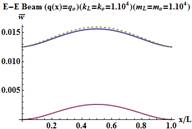
Fig. 3. Deflections in an E-E beam based on the two beam theories
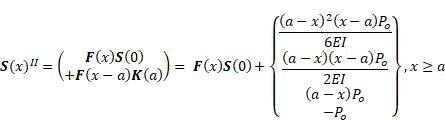
4. Solutions for a point force
In this section, due to the space
limitations, beams are assumed to be subjected to only a concentrated force ![]() acting at
acting at ![]() ,
, ![]() . Under this
assumption, the general solution is written before and after
. Under this
assumption, the general solution is written before and after ![]() as follows
as follows
|
|
The unknown elements of ![]() of
a C-E Euler-Bernoulli beam are to be
of
a C-E Euler-Bernoulli beam are to be
|
|
The unknown elements of the initial state
vector of an E-E Euler-Bernoulli beam are achieved as follows (![]()
|
|
||||
|
|
With the help of Eqs. (14)-(16), cross-sectional quantities at any section may be obtained.
5. Verifications of the results
Ghannadias and
Golmogany [5] presented a sextic B-spline method for the
numerical bending solution of a Euler-Bernoulli beam (We use article “a” here
because Euler is pronounced “yuler” I do believe) with arbitrary boundary
conditions on an elastic Winkler foundation. For an E-E beam under a uniformly
distributed force, the following properties are used in this work ![]() [5]:
[5]: ![]() ,
,
![]() ,
,
![]()
![]() .
Results are presented in Tables 3 and 4. From those
tables, a perfect harmonization is observed between the results.
.
Results are presented in Tables 3 and 4. From those
tables, a perfect harmonization is observed between the results.
Table 3
Validation of the present results of an E-E beam under uniformly distributed forces
|
|
[5]/Analitik |
[5]/B.Spline |
Present |
[5]/Analitik |
[5]/B.Spline |
Present |
|
x [cm] |
Displacement [cm] |
Slope [rad] |
||||
|
0. |
1.5 |
1.5 |
1.5 |
–0.00583 |
–0.00583 |
–0.00583 |
|
50. |
1.78596 |
1.78596 |
1.78596 |
–0.00550352 |
–0.00550352 |
–0.00550352 |
|
100. |
2.04102 |
2.04102 |
2.04102 |
–0.00461736 |
–0.00461736 |
–0.00461736 |
|
150. |
2.2407 |
2.2407 |
2.2407 |
–0.00331144 |
–0.00331144 |
–0.00331144 |
|
200. |
2.3675 |
2.3675 |
2.3675 |
–0.00172568 |
–0.00172568 |
–0.00172568 |
|
250. |
2.41093 |
2.41094 |
2.41094 |
0. |
0. |
0. |
|
300. |
2.3675 |
2.3675 |
2.3675 |
0.00172568 |
0.00172568 |
0.00172568 |
|
500. |
1.5 |
1.5 |
1.5 |
0.00583 |
0.00583 |
0.00583 |
|
x [cm] |
Bending moment [kgcm] |
Shear force [kg] |
||||
|
0. |
0. |
0. |
0. |
3750. |
3750. |
3750. |
|
50. |
168750. |
168750. |
168750. |
3000. |
3000. |
3000. |
|
100. |
300000. |
300000. |
300000. |
2250. |
2250. |
2250. |
|
150. |
393750. |
393750. |
393750. |
1500. |
1500. |
1500. |
|
200. |
450000. |
450000. |
450000. |
750. |
750. |
750. |
|
250. |
468750. |
468750. |
468750. |
0. |
0. |
0. |
|
300. |
450000. |
450000. |
450000. |
–750. |
–750. |
–750. |
|
500. |
0. |
0. |
0. |
–3750. |
–3750. |
–3750. |
Table 4
Variation of the maximum displacement (cm) in an E-E beam with the length of the beam
|
|
|
|||
|
100 |
250 |
500 |
1000 |
|
|
Present |
0.301457 |
0.806934 |
2.41094 |
17.575 |
|
B. spline [5] |
– |
– |
2.41094 |
– |
Let us show that
the elastic supports return to the rigid ones when very stiff springs are used.
The maximum dimensionless displacement in a C-E beam occurs at the mid-span
when very stiff springs are used (Table 5). Based on the Euler-
-Bernoulli beam theory, the maximum dimensionless displacement is evaluated as ![]() being insensitive to
the variation of the ratio of
being insensitive to
the variation of the ratio of ![]() as seen from Table 5.
This value is also equal to the maximum dimensionless displacement in a C-C
beam. The reason is that very stiff springs may behave as rigid supports.
as seen from Table 5.
This value is also equal to the maximum dimensionless displacement in a C-C
beam. The reason is that very stiff springs may behave as rigid supports.
|
|
|
Table 5
The maximum displacement in a C-E beam with very stiff springs under uniform forces
|
|
|
|
|
|
|
|
|
|||
|
Timoshenko |
0.00292917 |
0.00268542 |
0.00261717 |
0.00260742 |
|
Euler-Bernoulli |
0.00260417 |
0.00260417 |
0.00260417 |
0.00260417 |
Some other numerical displacements of this example in both dimensional and dimensionless form are also presented in Table 6 to provide insight into the problem. From this table, it is understood that the dimensionless displacements in a C-E Euler-Bernoulli beam with highly stiff springs, viz., in a C-C Euler-Bernoulli beam are insensitive to the ratio of length to the thickness. This does not mean that Euler-Bernoulli beam dimensional results do not change with the length of the beam.
Table 7 shows the dimensional
transverse displacements in a C-E beam with soft springs. This table states
that an Euler Bernoulli-beam with elastic supports may be sensitive to the ![]() ratios contrary to the classical supports. As expected, dimensional
displacements increase with increasing
ratios contrary to the classical supports. As expected, dimensional
displacements increase with increasing ![]() ratios. From Table 2,
however, their dimensionless counterparts decrease with increasing
ratios. From Table 2,
however, their dimensionless counterparts decrease with increasing ![]() ratios.
ratios.
Table 6
Both the dimensional and dimensionless displacements in a C-E beam with very stiff springs
|
|
|
|
|
|
|
x/L |
DIMENSIONLESS DISPLACEMENT, |
|||
|
0.2 |
0.00127467 |
0.00111867 |
0.00107499 |
0.00106875 |
|
0.6 |
0.002712 |
0.002478 |
0.00241248 |
0.00240312 |
|
1. |
1.25·10–22 |
7.8125·10–24 |
2·10–25 |
1.25·10–26 |
|
|
DIMENSIONLESS DISPLACEMENT, |
|||
|
0.2 |
0.00106667 |
0.00106667 |
0.00106667 |
0.00106667 |
|
0.6 |
0.0024 |
0.0024 |
0.0024 |
0.0024 |
|
1. |
1.25·10–22 |
7.8125·10–24 |
2·10–25 |
1.25·10–26 |
|
|
DIMENSIONAL DISPLACEMENT (m), |
|||
|
0.2 |
5.09867·10-6 |
0.0000715947 |
0.00268747 |
0.0427499 |
|
0.6 |
0.000010848 |
0.000158592 |
0.0060312 |
0.0961248 |
|
1. |
5·10–25 |
5·10–25 |
5·10–25 |
5·10–25 |
|
|
DIMENSIONAL DISPLACEMENT (m), |
|||
|
0.2 |
4.26667·10-6 |
0.0000682667 |
0.00266667 |
0.0426667 |
|
0.6 |
9.6·10-6 |
0.0001536 |
0.006 |
0.096 |
|
1. |
5·10–25 |
5·10–25 |
5·10–25 |
5·10–25 |
Table 7
The dimensional displacements in a C-E beam with soft springs
|
|
|
|
|
|
|
x/L |
DIMENSIONAL DISPLACEMENT (m), |
|||
|
0.2 |
9.29273·10–6 |
0.0000769821 |
0.00269294 |
0.0427553 |
|
0.6 |
0.0000360659 |
0.000191462 |
0.00606478 |
0.0961584 |
|
1. |
0.0000384507 |
0.0000490153 |
0.000049974 |
0.0000499984 |
|
|
DIMENSIONAL DISPLACEMENT (m), |
|||
|
0.2 |
8.31403·10–6 |
0.0000736139 |
0.00267213 |
0.0426721 |
|
0.6 |
0.000034687 |
0.000186484 |
0.00603358 |
0.0960336 |
|
1. |
0.0000381883 |
0.0000490077 |
0.000049974 |
0.0000499984 |
6. Conclusions
In the present study, some remarkable formulas were originally proposed for the bending behaviour of elastically supported Euler-Bernoulli beams under both uniformly distributed and concentrated loads via the transfer matrix approach. Dimensional and dimensionless results given in both tabular and graphical forms were discussed. It is mainly observed that Euler-Bernoulli beam solutions become sensitive to L/h ratios when they are elastically if it is elastically supported. The author hopes that these formulas will be quite useful when trying to validate purely computational solutions.
References
[1] Wang, C. (1995). Timoshenko beam-bending solutions in terms of Euler-Bernoulli solutions. Journal of Engineering Mechanics, 121(6), 763-765.
[2] Young, W.C. & Budynas, R.G. (2002). Roark’s Formulas for Stress and Strain, Seventh Edition, McGraw-Hill, New York, ISBN 0-07-072542-X.
[3] Mohammadi, R. (2014). Sextic B-spline collocation method for solving Euler-Bernoulli beam models. Applied Mathematics and Computation, 241, 151-166.
[4] Zamorska, I. (2014). Solution of differential equation for the Euler-Bernoulli beam. Journal of Applied Mathematics and Computational Mechanics, 13(4), 157-162.
[5] Ghannadiasl, A, & Golmogany, M.Z. (2017). Analysis of Euler-Bernoulli Beams with arbitrary boundary conditions on Winkler foundation using a B-spline collocation method. Engng. Trans., 65(3), 423-445.
[6] İnan, M. (1968). The Method of Initial Values and the Carry-over Matrix in Elastomechanics. ODTÜ Publication, Ankara, No: 20.
[7] Arici, M., & Granata, M.F. (2011). Generalized curved beam on elastic foundation solved by transfer matrix method. Structural Engineering & Mechanics, 40(2), 279-295.
[8] Wimmer, H., & Nachbagauer, K. (2018). Exact transfer- and stiffness matrix for the composite beam-column with Refined Zigzag kinematics. Composite Structures, 189, 700-706.
[9] Yıldırım, V. (2018). Several stress resultant and deflection formulas for Euler-Bernoulli beams under concentrated and generalized power/sinusoidal distributed loads. International Journal of Engineering & Applied Sciences (IJEAS), 10(2), 35-63. DOI: 10.24107/ijeas.430666.