The Sturm-Liouville eigenvalue problem - a numerical solution using the Control Volume Method

• BibTex
• RIS
• APA
• Harvard
• IEEE
• MLA
• Vancouver
• Chicago

@article{Siedlecki_2016,
   doi = {10.17512/jamcm.2016.2.14},
   url = {https://doi.org/10.17512/jamcm.2016.2.14},
   year = 2016,
   publisher = {The Publishing Office of Czestochowa University of Technology},
   volume = {15},
   number = {2},
   pages = {127--136},
   author = {Jarosław Siedlecki and  Mariusz Ciesielski and  Tomasz Błaszczyk},
   title = {The Sturm-Liouville eigenvalue problem - a numerical solution using the Control Volume Method},
   journal = {Journal of Applied Mathematics and Computational Mechanics}
}

TY  - JOUR
DO  - 10.17512/jamcm.2016.2.14
UR  - https://doi.org/10.17512/jamcm.2016.2.14
TI  - The Sturm-Liouville eigenvalue problem - a numerical solution using the Control Volume Method
T2  - Journal of Applied Mathematics and Computational Mechanics
JA  - J Appl Math Comput Mech
AU  - Siedlecki, Jarosław
AU  - Ciesielski, Mariusz
AU  - Błaszczyk, Tomasz
PY  - 2016
PB  - The Publishing Office of Czestochowa University of Technology
SP  - 127
EP  - 136
IS  - 2
VL  - 15
SN  - 2299-9965
SN  - 2353-0588
ER  - 

Siedlecki, J., Ciesielski, M., & Błaszczyk, T. (2016). The Sturm-Liouville eigenvalue problem - a numerical solution using the Control Volume Method. Journal of Applied Mathematics and Computational Mechanics, 15(2), 127-136. doi:10.17512/jamcm.2016.2.14

Siedlecki, J., Ciesielski, M. & Błaszczyk, T., 2016. The Sturm-Liouville eigenvalue problem - a numerical solution using the Control Volume Method. Journal of Applied Mathematics and Computational Mechanics, 15(2), pp.127-136. Available at: https://doi.org/10.17512/jamcm.2016.2.14

[1]J. Siedlecki, M. Ciesielski and T. Błaszczyk, "The Sturm-Liouville eigenvalue problem - a numerical solution using the Control Volume Method," Journal of Applied Mathematics and Computational Mechanics, vol. 15, no. 2, pp. 127-136, 2016.

Siedlecki, Jarosław, Mariusz Ciesielski, and Tomasz Błaszczyk. "The Sturm-Liouville eigenvalue problem - a numerical solution using the Control Volume Method." Journal of Applied Mathematics and Computational Mechanics 15.2 (2016): 127-136. CrossRef. Web.

1. Siedlecki J, Ciesielski M, Błaszczyk T. The Sturm-Liouville eigenvalue problem - a numerical solution using the Control Volume Method. Journal of Applied Mathematics and Computational Mechanics. The Publishing Office of Czestochowa University of Technology; 2016;15(2):127-136. Available from: https://doi.org/10.17512/jamcm.2016.2.14

Siedlecki, Jarosław, Mariusz Ciesielski, and Tomasz Błaszczyk. "The Sturm-Liouville eigenvalue problem - a numerical solution using the Control Volume Method." Journal of Applied Mathematics and Computational Mechanics 15, no. 2 (2016): 127-136. doi:10.17512/jamcm.2016.2.14

THE STURM-LIOUVILLE EIGENVALUE PROBLEM - A NUMERICAL SOLUTION USING THE CONTROL VOLUME METHOD

Jarosław Siedlecki¹, Mariusz Ciesielski², Tomasz Błaszczyk¹

¹Institute of Mathematics, Czestochowa University of Technology
Częstochowa, Poland
²Institute of Computer and Information Sciences
Czestochowa University of Technology, Częstochowa, Poland
jaroslaw.siedlecki@im.pcz.pl, mariusz.ciesielski@icis.pcz.pl, tomasz.blaszczyk@im.pcz.pl

Abstract. The solution of the 1D Sturm-Liouville problem using the Control Volume Method is discussed. The second order linear differential equation with homogeneous boundary conditions is discretized and converted to the system of linear algebraic equations. The matrix associated with this system is tridiagonal and eigenvalues of this system are an approximation of the real eigenvalues of the boundary value problem. The numerical results of the eigenvalues for various cases and the experimental rate of convergence are presented.

Keywords: Sturm-Liouville problem, eigenvalues, numerical methods, Control Volume Method

1. Introduction

This paper is concerned with the computation of eigenvalues of regular eigenvalue problems occurring in ordinary differential equations. The Sturm-Liouville problem arises within in many areas of science, engineering and applied mathematics. It has been studied for more than two decades. Many physical, biological and chemical processes are described using models based on the Sturm-Liouville equations.

The Sturm-Liouville problem appears directly as the eigenvalue problem in a one-dimensional space. It also arises when linear partial differential equations are separable in a certain coordinate system. For a more detailed study of the integer order Sturm-Liouville theory, we refer the reader to [1-5].

The Sturm-Liouville problem can be solved by using either analytical or numerical methods. One of the most common approaches to a numerical solution of the considered problem is the finite difference method [3, 6-8] where each derivative is discretized at each grid point with an adequate difference scheme. Apart from the finite difference method, several analytical ones, such as the variational or decomposition methods, are proposed to find an approximate solution.

2. Statement of the problem

We consider the following problem defined on the bounded interval x [a, b]

(1)

(2)

where p(x) > 0, dp/dx and q(x) are continuous, w(x) > 0 on [a, b], and . The above problem is called the regular Sturm-Liouville Problem (SLP). The solution to SLP consists of a pair l and y, where l is a constant - called an eigenvalue, while y is a nontrivial (nonzero) function - called an eigenfunction, and together they satisfy the given SLP. For each SLP, the eigenvalues form an infinite increasing sequence: l₁ < l₂ < l₃ < … and lim_k®¥l_k = ¥.

For arbitrary choices of the functions p(x), q(x) and w(x) in Eq. (1), the computation of the exact values of the eigenvalues for which SLP (1)-(2) has a nontrivial eigensolution y(x) which is very complicated or it is practically impossible to determine. Numerical methods should, therefore, be used for computing the approximate values of l. In many cases, the importance of a numerical approximation to the SLP described by a differential eigenvalue problem is to reduce the problem to that of solving the eigenvalue problem of a matrix equation (an algebraic problem).

In this paper, we apply the Control Volume Method (also known as the Finite Volume Method) to compute the eigenvalues of the Sturm-Liouville problem numerically.

3. Control Volume Method

In this numerical method [9] the considered domain of SLP: x [a, b] is divided into N control volumes W_i for i = 1,…,N with the central nodes x_i. The mesh is presented in Figure 1. The auxiliary nodes x_i = a + i Dx, for i = 0,…,N and Dx = = (b - a) / N have also been introduced. Then, the positions of central nodes are the following: x_i = a + (i - 0.5)Dx, i = 1,…,N.

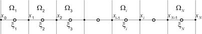
Fig. 1. Mesh of control volumes

The integration of Eq. (1) with respect to volume W_i leads to

(3)

or written in the form (assuming that W_i: [x_i-1, x_i])

(4)

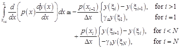
All the components in Eq. (4) can be approximated as follows:

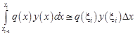(5)

(6)

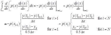(7)

The values of y_a = y(a) and y_b = y(b) are determined on the basis of approximations of the boundary conditions (2)

(8)

and hence, these values are equal to

(9)

Substituting (9) into (8), the following approximation of (7) has been obtained

(10)

where

,

(11)

For example, in the case of the Dirichlet boundary conditions at boundaries x = a (i.e. a₁ = 1, a₂ = 0) and/or x = b (i.e. b₁ = 1, b₂ = 0), the coefficients g_a and g_b are equal to 2, and in the case of the Neumann boundary conditions at x = a (a₁ = 0, a₂ = 1) and/or x = b (b₁ = 0, b₂ = 1), these coefficients take the values of 0, respectively.

After substitution of (5), (6) and (10) into (4), the following system of the discrete equations for every control volume:

· for W₁:

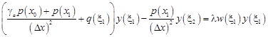(12)

· for W_i, for i = 2,…,N - 1:

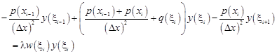(13)

· for W_N:

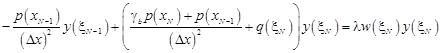(14)

is obtained.

This system can be also written in the matrix form as

(15)

where

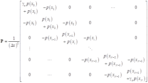(16)

(17)

(18)

and . Then, SLP (1)-(2) is equivalent to the matrix eigenvalue problem (15). The ordered eigenvalues of (15) are denoted by l_i^(N), i = 1,…,N.

In order to evaluate eigenvalues of large matrix eigenvalue problem (15), the numerical methods implemented in mathematical software can be used.

3.1. Particular case

Assuming the functions p(x) = 1, q(x) = 0 and w(x) = 1 in the SLP problem, then matrices P, Q and W are reduced to the following forms: Q = O (Zero matrix), W = I (Identity matrix) and

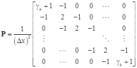(19)

In the case of the mixed Dirichlet and/or Neumann boundary conditions at both boundaries, one can find in literature (e.g. [4]) the explicit formulas for the i-th eigenvalue l_i of the SLP (1)-(2) and they are presented in Table 1. For the discrete case, the eigenvalues of the matrix P can be determined in an analytical way. The eigenvalue problems of tridiagonal matrices (in a similar form as the matrix P) are considered in [10, 11]. On the basis of these results, the eigenvalues of the matrix P: l_i^(N), i = 1,…,N are adopted to the analysed problem for four mixed boundary conditions and they are also given in Table 1.

Table 1

Eigenvalues of Eq. (1) for functions p(x) = 1, q(x) = 0 and w(x) = 1 and four mixed cases of boundary conditions (explicit formulas for l_i, i = 1,…,∞ and discrete one for l_i^(N), i = 1,…,N )

For more complicated cases such as non-constant functions p(x), q(x), w(x) occurring in Eq. (1), the eigenvalues of system (15) should be determined in a numerical way (i.e. using mathematical software - here the Maple is used).

3.2. Error of numerical approximation of the eigenvalues

Theorem 1. For the Sturm-Liouville problem (1)-(2) there exists a constant C such that the i-th exact eigenvalue l_i and the approximate eigenvalue l_i^(N) satisfy the following relation

(20)

Proof: For the presented formulas in Table 1 (in these cases, the exact and discrete eigenvalues are known), one can estimate the error of approximation of the discrete eigenvalues. Let us start from the Taylor series expansion for the function sin²(x) at about point x = 0

(21)

Next, if we take into account the first two terms in the Taylor series (21), then we estimate the following expression as

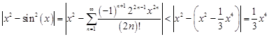(22)

For the case of the Dirichlet-Dirichlet boundary conditions, the error is evaluated by using the estimation (22) in the following way:

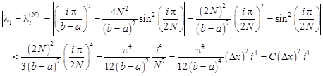(23)

In the other cases (from Table 1), the results are similar.

Another method of error estimation is based on the investigation of the Experimental Rate of Convergence (ERC). The total error in the estimate of the eigenvalues is composed of both the error resulting from the discretization of the equation and the error of the numerical algorithm for finding eigenvalues of system (15). Here, we assume that the error is

(24)

where the parameters r and s are to be determined experimentally.

If the i-th exact eigenvalue l to SLP is known, then the parameters r and s can be determined using the following formulas for the ERC for variable values of N:

(25)

(26)

Whereas, if the exact eigenvalue is unknown then, we determine the parameter r from the following formula

(27)

The parameter s can be estimated using (26) and assuming that l_i is numerically determined for sufficiently high value of N.

4. Example of numerical simulations

In tests of verification of the numerical solutions, three cases are taken into account:

· Example 1: p(x) = 1, q(x) = 0, w(x) = (1 + x)^‒2, a₁ = 1, a₂ = 0, b₁ = 1, b₂ = 0.

· Example 2: p(x) = (x + 1)², q(x) = x² - 2, w(x) = exp(x), a₁ = 1, a₂ = 0, b₁ = 0, b₂ = 1.

· Example 3: p(x) = 2 + sin(2px), q(x) = -10, w(x) = 1 + sqrt(x), a₁ = 1, a₂ = 0, b₁ = 5, b₂ = 1.

In all examples, the values of a = 0 and b = 1 have been assumed.

In the case of Example 1, the exact eigenvalues are given by [12], while for the remaining cases the exact eigenvalues are unknown.

In Tables 2, 4 and 5, the numerical values of the first 8 eigenvalues for different values of N and the calculated ERC_r ((25) or (27)) for all examples are presented, respectively. In addition, in Table 3, the calculated values of ERC_s (26) for Example 1 are shown.

Table 2

Eigenvalues and ERC_r for Example 1

Table 3

ERC_s for Example 1

Table 4

Eigenvalues and ERC_r for Example 2

Table 5

Eigenvalues and ERC_r for Example 3

The analysis of the results presented in Tables 2-5 indicates that the rate r (ERC_r) is close to 2, while the rate s (ERC_s) is close to 4. Thus we can confirm that the relationship (20) is satisfied. The errors in the approximation of eigenvalues increase rapidly as the index of the eigenvalue grows.

5. Conclusions

In this paper, the new approach based on the control volume method for finding the eigenvalues of the Sturm-Liouville problem was discussed. The continuous problem described by the differential equation with the adequate boundary conditions was converted to the corresponding discrete one. The rate of convergence of the proposed numerical scheme is order 2. The presented results of the approximation of eigenvalues are in close agreement with the results obtained in an analytical way or in the mathematical software field. In the future, the presented approach can be extended to apply high order of accuracy difference schemes for approximating eigenvalues of the Sturm-Liouville problem and can be applied to the fractional Sturm-Liouville problem which is related to the corresponding fractional Euler-‑Lagrangian equation [13].

References

[1] Agarwal R.P., O’Regan D., An Introduction to Ordinary Differential Equations, Springer, New York 2008.

[2] Atkinson F.V., Discrete and Continuous Boundary Value Problems, Academic Press, New York, London 1964.

[3] Pryce J.D., Numerical Solution of Sturm-Liouville Problems, Oxford Univ. Press, London 1993.

[4] Zaitsev V.F., Polyanin A.D., Handbook of Exact Solutions for Ordinary Differential Equations, CRC Press, New York 1995.

[5] Pruess S., Estimating the eigenvalues of Sturm-Liouville problems by approximating the differential equation, SIAM J. Numer. Anal. 1973, 10, 55-68.

[6] Aceto L., Ghelardoni P., Magherini C., Boundary value methods as an extension of Numerov’s method for Sturm-Liouville eigenvalue estimates, Applied Numerical Mathematics 2009, 59 (7), 1644-1656.

[7] Amodio P., Settanni G., A matrix method for the solution of Sturm-Liouville problems, Journal of Numerical Analysis, Industrial and Applied Mathematics (JNAIAM) 2011, 6 (1-2), 1-13.

[8] Ascher U.M., Numerical Methods for Evolutionary Differential Equations, SIAM, 2008.

[9] Ascher U.M., Mattheij R.M.M., Russell R.D., Numerical Solution of Boundary Value Problems for ODEs, Classics in Applied Mathematics 13, SIAM, Philadelphia 1995.

[10] Elliott J.F., The characteristic roots of certain real symmetric matrices, Master’s Thesis, University of Tennessee, 1953.

[11] Gregory R.T., Karney D., A Collection of Matrices for Testing Computational Algorithm, Wiley-Interscience, 1969.

[12] Akulenko L.D., Nesterov S.V., High-Precision Methods in Eigenvalue Problems and Their Applications (series: Differential and Integral Equations and Their Applications), Chapman and Hall/CRC, 2004.

[13] Ciesielski M., Blaszczyk T., Numerical solution of non-homogenous fractional oscillator equation in integral form, Journal of Theoretical and Applied Mechanics 2015, 53 (4), 959-968.

[14] Press W.H., Teukolsky S.A., Vetterling W.T., Flannery B.P., Numerical Recipes: The Art of Scientific Computing (3rd ed.), Cambridge University Press, New York 2007.