Trefftz method for an inverse geometry problem in steady-state heat conduction
Leszek Hożejowski
Journal of Applied Mathematics and Computational Mechanics |
 Download Full Text |
 View in HTML format |
 Export citation |
@article{Hożejowski_2016,
   doi = {10.17512/jamcm.2016.2.05},
   url = {https://doi.org/10.17512/jamcm.2016.2.05},
   year = 2016,
   publisher = {The Publishing Office of Czestochowa University of Technology},
   volume = {15},
   number = {2},
   pages = {41--52},
   author = {Leszek Hożejowski},
   title = {Trefftz method for an inverse geometry problem in steady-state heat conduction},
   journal = {Journal of Applied Mathematics and Computational Mechanics}
}
TY - JOUR DO - 10.17512/jamcm.2016.2.05 UR - https://doi.org/10.17512/jamcm.2016.2.05 TI - Trefftz method for an inverse geometry problem in steady-state heat conduction T2 - Journal of Applied Mathematics and Computational Mechanics JA - J Appl Math Comput Mech AU - Hożejowski, Leszek PY - 2016 PB - The Publishing Office of Czestochowa University of Technology SP - 41 EP - 52 IS - 2 VL - 15 SN - 2299-9965 SN - 2353-0588 ER -
Hożejowski, L. (2016). Trefftz method for an inverse geometry problem in steady-state heat conduction. Journal of Applied Mathematics and Computational Mechanics, 15(2), 41-52. doi:10.17512/jamcm.2016.2.05
Hożejowski, L., 2016. Trefftz method for an inverse geometry problem in steady-state heat conduction. Journal of Applied Mathematics and Computational Mechanics, 15(2), pp.41-52. Available at: https://doi.org/10.17512/jamcm.2016.2.05
[1]L. Hożejowski, "Trefftz method for an inverse geometry problem in steady-state heat conduction," Journal of Applied Mathematics and Computational Mechanics, vol. 15, no. 2, pp. 41-52, 2016.
Hożejowski, Leszek. "Trefftz method for an inverse geometry problem in steady-state heat conduction." Journal of Applied Mathematics and Computational Mechanics 15.2 (2016): 41-52. CrossRef. Web.
1. Hożejowski L. Trefftz method for an inverse geometry problem in steady-state heat conduction. Journal of Applied Mathematics and Computational Mechanics. The Publishing Office of Czestochowa University of Technology; 2016;15(2):41-52. Available from: https://doi.org/10.17512/jamcm.2016.2.05
Hożejowski, Leszek. "Trefftz method for an inverse geometry problem in steady-state heat conduction." Journal of Applied Mathematics and Computational Mechanics 15, no. 2 (2016): 41-52. doi:10.17512/jamcm.2016.2.05
TREFFTZ METHOD FOR AN INVERSE GEOMETRY PROBLEM IN STEADY-STATE HEAT CONDUCTION
Leszek Hożejowski
Department of Computer Science and
Applied Mathematics, Kielce University of Technology
Kielce, Poland
hozej@tu.kielce1.pl
Abstract. The paper addresses a boundary identification problem in two-dimensional steady-state heat conduction. The proposed approach based on the Trefftz method allows one to reconstruct the unknown part of a regular domain boundary from the given temperature measurements on it, provided that both the temperature and heat flux on the remaining part of the boundary are known. The reconstruction of an unknown boundary is done through successive approximations with a polynomial or a truncated Fourier series. The proposed solution method, whose merit lies in the avoidance of large systems of nonlinear equations, is fast converging, accurate and numerically stable, as demonstrated in the included numerical examples.
Keywords: inverse geometry problem, boundary identification, Trefftz method
1. Introduction
An important category of problems considered in science and engineering are inverse problems. When the system geometry is not fully known but is being investigated, such problems are referred to as inverse geometry problems (IGPs). Some typical examples could be determining a moving interface between liquid and solid phases or nondestructive detection of internal cracks or cavities in materials. According to the classification proposed in [1], inverse analysis concerning IGPs can be applied to problems related to (i) shape and design optimization, (ii) identification of defects and (iii) identification of an unknown part of the boundary. The paper focuses attention on the latter.
Most of the studies concerning this task are devoted to problems described by Laplace’s equation. As known, Laplace’s equation characterizes a large group of physical problems. The present study refers specifically to steady-state isotropic heat conduction.
Numerical reconstruction of the unknown boundary can be achieved by a variety of computational approaches, e.g. the radial basis functions method [2], the boundary element regularization method [3], the smoothed grid finite element method [4] or the level set method [5] - to name a few. As the present study employs the Trefftz method, we focus particular attention to the approaches applying this method or related techniques. The modified collocation Trefftz method for a boundary detection problem was used in [6, 7] and the same technique was applied for an inverse geometric problem governed by the biharmonic equation [8] and the modified Helmholtz equation [9]. The regularized collocation Trefftz approach was successfully tested on different shapes in a two-dimensional void detection problem [10]. The method of fundamental solutions, which may be viewed as one of the Trefftz methods, also belongs to computational techniques effective in IGPs, see e.g. [11, 12].
The cited references concerning the solution of a boundary identification problem by the (modified) collocation Trefftz method propose a discrete reconstruction of an unknown boundary. In contrast, the present study uses a polynomial or a Fourier expansion of the unknown boundary. The computational procedure first outputs the solution of Laplace’s equation by the Trefftz method. The further step consists in specification of the coefficients of a polynomial or a Fourier representation of the unknown boundary so as to best fit the calculated temperatures to their known values. The latter requires solving systems of nonlinear algebraic equations but with relatively few unknowns which is the specific value of the approach.
2. Boundary identification problem
We consider a problem in a finite two-dimensional
region ![]() whose boundary
whose boundary ![]() is
composed of two disjoint curves
is
composed of two disjoint curves ![]() and
and![]() :
:
| (1) |
such that ![]() is
known and
is
known and ![]() unknown. Highly irregular shapes of
unknown. Highly irregular shapes of ![]() will not be addressed in this paper as
they usually require a division into subdomains and local solutions, while the
present approach uses global Trefftz-type solutions which could fail in complex
geometries. We assume that
will not be addressed in this paper as
they usually require a division into subdomains and local solutions, while the
present approach uses global Trefftz-type solutions which could fail in complex
geometries. We assume that ![]() is smooth and can be
described by a function
is smooth and can be
described by a function ![]() or
or ![]() , depending on the type of coordinates. In spite of these constraints on the
topology of
, depending on the type of coordinates. In spite of these constraints on the
topology of![]() , the proposed algorithm allows a great
variety of shapes occurring in real-world applications.
, the proposed algorithm allows a great
variety of shapes occurring in real-world applications.
The discussed problem is that of stationary heat flow with no heat sources or sinks, so the governing equation is
| (D - Laplace operator) (2) |
which we solve subject to
| (3) |
| (4) |
where ![]() denotes differentiation along the outward normal n.
Equations (3) and (4) represent an overspecified condition on
denotes differentiation along the outward normal n.
Equations (3) and (4) represent an overspecified condition on ![]() (known temperature and
heat flux) in order to compensate for the missing information concerning
geometric characteristics of the problem domain. On the remaining (unknown)
part of the boundary, we impose a Dirichlet condition:
(known temperature and
heat flux) in order to compensate for the missing information concerning
geometric characteristics of the problem domain. On the remaining (unknown)
part of the boundary, we impose a Dirichlet condition:
| (5) |
with ![]() not necessarily constant. Since
not necessarily constant. Since ![]() is being sought, condition (5) should be understood as
a given temperature at the points
is being sought, condition (5) should be understood as
a given temperature at the points ![]() or
or ![]() whose first coordinates are known while
second coordinates are to be found.
whose first coordinates are known while
second coordinates are to be found.
3. Trefftz method
The Trefftz method, developed at the end of the 1920s, has recently become very popular. It approximates the solution of a differential equation with a linear combination of certain basis functions (named T-complete functions) satisfying the given differential equation. For Laplace’s equation in (x, y)-coordinates, the proper basis is composed of the functions commonly known as harmonic polynomials:
| (6) |
In polar coordinates the corresponding basis functions are
| (7a) |
unless for to a problem in a multiple domain, when we use the bases:
| (7b) |
According to the logic of the Trefftz method,
the approximate solution of (2)-(5), denoted ![]() , can
be written as a linear combination of the form
, can
be written as a linear combination of the form
| (8) |
with ![]() denoting the T-complete
functions of type (6), (7a) or (7b) and
denoting the T-complete
functions of type (6), (7a) or (7b) and ![]() - the coefficients
to be found. In order to specify the coefficients
- the coefficients
to be found. In order to specify the coefficients ![]() we
minimize
a functional
we
minimize
a functional
 | (9) |
which leads to a system of linear equations:
| (10) |
4. Boundary identification algorithm
The problem of identification of an unknown boundary g can be set up in terms of searching for either (x, y)- or (r, θ)-coordinates of the boundary points. Regardless of chosen coordinates, the proposed solution scheme assumes reconstruction of a boundary through its approximation by a function whose parameters need to be specified. The advantage of such an approach lies in reducing computational effort as we are able to recover infinitely many boundary points at the cost of finding only a few parameters of an approximating curve.
The boundary identification algorithm further described in this section can be summarized as follows:
STEP 1.
Approximate the temperature T of a considered body with ![]() , using the Trefftz method.
, using the Trefftz method.
STEP 2. Choose the form of an approximation to g : with a
polynomial ![]() or a finite
trigonometric series
or a finite
trigonometric series ![]() .
.
STEP 3. Choose ![]() - the demanded level of accuracy in approximation of the given
- the demanded level of accuracy in approximation of the given ![]() on
on ![]() by
by ![]() on
the graph of
on
the graph of ![]() /or
/or ![]() .
.
STEP 4. Specify the coefficients of ![]() /or
/or ![]() for
for ![]() . If the
required accuracy
. If the
required accuracy ![]() is achieved with
is achieved with ![]() /or
/or ![]() , stop. Otherwise go to STEP 5.
, stop. Otherwise go to STEP 5.
STEP 5. Increase N by 1. Then
specify the coefficients of ![]() /or
/or ![]() .
If the required accuracy
.
If the required accuracy ![]() is achieved with
is achieved with ![]() /or
/or ![]() ), stop.
Otherwise
repeat STEP 5.
), stop.
Otherwise
repeat STEP 5.
4.1. Implementation in (x, y)-coordinates
In the considered problem we assume that ![]() is a smooth curve
is a smooth curve ![]() which we can approximate with an Nth
degree polynomial:
which we can approximate with an Nth
degree polynomial:
| (11) |
By construction, ![]() has to agree with
has to agree with ![]() at both ends (corresponding to
at both ends (corresponding to ![]() and
and ![]() ),
hence to determine
),
hence to determine ![]() coefficients of the polynomial
coefficients of the polynomial![]() , we
do not need to solve
, we
do not need to solve ![]() equations but only
equations but only![]() .
.
Condition (5), when expressed in terms of approximate functions, gives
| (12) |
which holds
in the whole interval [a, b] or at M selected points ![]() .
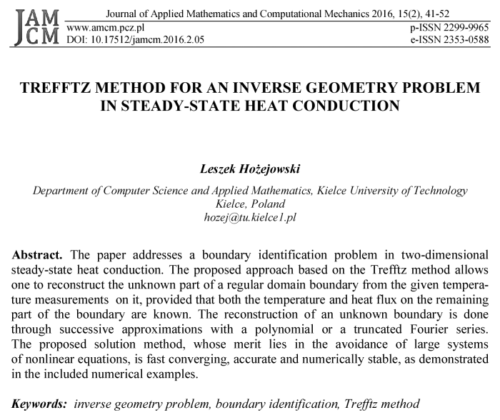
In general, such a condition cannot be met in the strict sense,
therefore we claim fulfilment in a variational sense, i.e. seeking the minimum
of a functional
.
In general, such a condition cannot be met in the strict sense,
therefore we claim fulfilment in a variational sense, i.e. seeking the minimum
of a functional
| (13) |
where ![]() denotes L2-norm
of a function or an M-dimensional vector. Minimization of
denotes L2-norm
of a function or an M-dimensional vector. Minimization of ![]() leads to a system of
nonlinear algebraic equations
leads to a system of
nonlinear algebraic equations
| (14) |
which we solve numerically. It is worth noting
that the Trefftz method itself can approximate temperature but not shape.
However, it is involved in polynomial boundary reconstruction through
delivering the temperature ![]() , which appears in
(13) and consequently in (14).
, which appears in
(13) and consequently in (14).
Once ![]() is
found, the polynomial approximations of
is
found, the polynomial approximations of ![]() will
be determined
in order of an increasing degree. Before further description of the procedure,
for
each polynomial
will
be determined
in order of an increasing degree. Before further description of the procedure,
for
each polynomial ![]() we define a nonnegative
number,
we define a nonnegative
number, ![]() , which measures
the relative error between the exact and calculated temperature on the unknown
boundary:
, which measures
the relative error between the exact and calculated temperature on the unknown
boundary:
 , , | (15) |
provided ![]() . At
the Nth step,
. At
the Nth step, ![]() will be compared with the maximum
admissible error,
will be compared with the maximum
admissible error, ![]() , chosen prior to computation.
The first reconstruction of
, chosen prior to computation.
The first reconstruction of![]() is with a polynomial
of the lowest degree (0 or 1). We check whether this initial
approximation, say
is with a polynomial
of the lowest degree (0 or 1). We check whether this initial
approximation, say ![]() , is sufficiently accurate, i.e. whether
, is sufficiently accurate, i.e. whether ![]() . If
so, we have the solution. Otherwise, we search for a polynomial of degree 2,
whose coefficients minimize (13) and unless
. If
so, we have the solution. Otherwise, we search for a polynomial of degree 2,
whose coefficients minimize (13) and unless ![]() , we
construct (in the same
manner) the next polynomial approximations of degree
, we
construct (in the same
manner) the next polynomial approximations of degree ![]() ,
until we achieve
,
until we achieve ![]() for some N. Note that
we derive the coefficients of
for some N. Note that
we derive the coefficients of ![]() ’s from nonlinear equations (14). Numerical
procedures for solving nonlinear equations usually need a certain initial
guess. If
’s from nonlinear equations (14). Numerical
procedures for solving nonlinear equations usually need a certain initial
guess. If ![]() , we plot
, we plot ![]() versus
versus ![]() in
order to suggest initial value for
in
order to suggest initial value for ![]() , while
, while ![]() and
and ![]() can
be expressed as functions of
can
be expressed as functions of![]() . For
. For ![]() , one can take the (N – 1)th
polynomial as an initial guess for finding the coefficients of the Nth
polynomial.
, one can take the (N – 1)th
polynomial as an initial guess for finding the coefficients of the Nth
polynomial.
4.2. Implementation in (r, φ)-coordinates
Described in polar coordinates, the unknown
boundary is assumed to be
the graph of a function ![]() . A reasonable
approximation of
. A reasonable
approximation of ![]() seems to be that by a finite
series of trigonometric functions:
seems to be that by a finite
series of trigonometric functions:
| (16) |
in which we admit ![]() from
0 to 2π. The adjustment of
from
0 to 2π. The adjustment of ![]() ’s
and
’s
and ![]() ’s runs similarly to the (x,y)
case, i.e. through minimization of a functional
’s runs similarly to the (x,y)
case, i.e. through minimization of a functional ![]() analogous
to (13). Finding
analogous
to (13). Finding ![]() requires more computation in
comparison to finding a polynomial
requires more computation in
comparison to finding a polynomial ![]() as we have to specify
as we have to specify ![]() parameters of the Nth
order approximation, whereas in (11) only
parameters of the Nth
order approximation, whereas in (11) only ![]() .
.
The start-up approximation of ![]() is of 0th
or 1st order. When
is of 0th
or 1st order. When ![]() , we first take
, we first take ![]() . Otherwise, we put
. Otherwise, we put ![]() and specify e.g.
and specify e.g. ![]() through plotting
through plotting ![]() versus
versus ![]() (while
(while
![]() and
and ![]() can
be expressed in terms of
can
be expressed in terms of![]() ). Further proceeding
runs similar to that described in Section 4.1.
). Further proceeding
runs similar to that described in Section 4.1.
5. Numerical results
In this section, we present a couple of numerical examples. The computations were performed on numerically simulated (synthetic) temperature, as in the reference papers [6-11]. Such an approach allows convenient and accurate evaluation of the results because the exact solution is known.
For better assessment of the solution method,
each example was based on
a different analytical solution to Laplace’s equation. The
measurements on ![]() were simulated
at M points uniformly distributed on the given range of x or
were simulated
at M points uniformly distributed on the given range of x or ![]() . We
assume the algorithm stops when
. We
assume the algorithm stops when ![]() attains ~10‒6. For
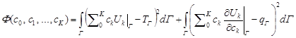
assessing the accuracy of boundary reconstruction in measurable terms, we
introduce the error
attains ~10‒6. For
assessing the accuracy of boundary reconstruction in measurable terms, we
introduce the error ![]() ,
defined by
,
defined by
 | (17) |
Example 1.
Let the problem domain be described by inequalities
| (18) |
where
| (19) |
will be the unknown boundary ![]() to be found.
The exact temperature is
to be found.
The exact temperature is ![]() . We take T-complete functions of the type (6)
with
. We take T-complete functions of the type (6)
with ![]() in the
expansion (8) and
in the
expansion (8) and ![]() . The problem
domain is presented
in Figure 1(a) and a polynomial reconstruction of
. The problem
domain is presented
in Figure 1(a) and a polynomial reconstruction of ![]() in Figure 1(b).
in Figure 1(b).
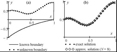
Fig. 1. Problem
domain ![]() (a) and boundary identification by a polynomial
of degree N = 8 (b)
(a) and boundary identification by a polynomial
of degree N = 8 (b)
Further evidence concerning accuracy and rate of convergence is given in Table 1.
Table 1
Errors for stopping criterion, ET(N), and errors of boundary detection, e(N)
|
N |
2 |
3 |
4 |
5 |
6 |
7 |
8 |
|
ET(N), (%) |
3.56 |
3.49 |
0.37 |
0.35 |
0.021 |
0.020 |
0.0008 |
|
e(N), (%) |
12.14 |
11.80 |
1.26 |
1.17 |
0.073 |
0.066 |
0.0027 |
The errors listed in Table 1 show high accuracy and fast convergence of the solution procedure as only few iterations were sufficient for very accurate reconstruction of the unknown boundary.
Example 2.
This example refers to a region defined (in polar coordinates) by inequalities
| (20) |
with
| (21) |
When constrained to ![]() ,
the function
,
the function ![]() will be the unknown
boundary to be identified. In this example we take
will be the unknown
boundary to be identified. In this example we take ![]() .
The considered case requires T-complete functions (7a). We take
.
The considered case requires T-complete functions (7a). We take ![]() in (8) and
in (8) and ![]() . Figure 2a shows the domain boundaries (known
and unknown) and Figure 2b compares the exact
. Figure 2a shows the domain boundaries (known
and unknown) and Figure 2b compares the exact ![]() with its approximation
corresponding to N = 8.
with its approximation
corresponding to N = 8.
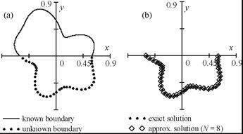
Fig. 2. Problem domain ![]() (a) and boundary identification by
expansion (16) with N = 8 (b)
(a) and boundary identification by
expansion (16) with N = 8 (b)
Table 2 provides with more information concerning convergence properties and accuracy of the algorithm.
Table 2
Errors for stopping criterion, ET(N), and errors of boundary detection, e(N)
|
N |
1 |
2 |
3 |
4 |
5 |
6 |
7 |
8 |
|
ET(N), % |
4.21 |
3.87 |
1.45 |
0.24 |
0.027 |
0.007 |
0.002 |
0.0002 |
|
e(N), % |
18.05 |
15.21 |
8.59 |
1.92 |
0.29 |
0.076 |
0.023 |
0.003 |
As in the previous example, we achieved very good accuracy of the boundary identification. Moreover, the small number of iterations before terminating the procedure indicates fast convergence.
Example 3.
We consider a doubly connected domain described in polar coordinates by
| (22) |
where
| (23) |
is its outer boundary where the temperature was known at M = 60 points and
| (24) |
is the unknown inner boundary. We generated the
measurements from ![]() . The suitable Trefftz-bases
for this example are those of type (7b) and we take
. The suitable Trefftz-bases
for this example are those of type (7b) and we take ![]() . Figure 3 presents the boundaries of
. Figure 3 presents the boundaries of ![]() and the approximation of
and the approximation of ![]() found by the algorithm.
found by the algorithm.
|
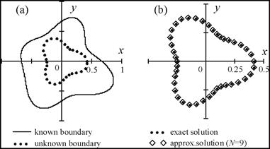
Fig. 3. Problem domain ![]() (a) and boundary identification by
expansion (16) with N = 9 (b)
(a) and boundary identification by
expansion (16) with N = 9 (b)
Table 3 includes information for assessing the obtained approximations.
Table 3
Errors for stopping criterion, ET(N), and errors of boundary detection, e(N)
|
N |
2 |
3 |
4 |
5 |
6 |
7 |
8 |
9 |
|
ET(N), % |
2.94 |
0.30 |
0.073 |
0.034 |
0.031 |
0.003 |
0.0012 |
0.0004 |
|
e(N), % |
20.09 |
1.68 |
0.466 |
0.235 |
0.236 |
0.023 |
0.014 |
0.0042 |
The present example, like the two already discussed, demonstrated very high accuracy of the final-order solution and fast convergence of the algorithm.
6. Sensitivity to input errors
The calculation was repeated using the input
data disturbed by random errors. For that purpose we generated M
normally distributed random numbers from
the range between ![]() and
and ![]() .
Such a level of noise was intended to create
realistic test data. The evaluation of the influence of those noisy inputs on
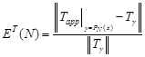
the final boundary reconstruction is through calculating a relative error
.
Such a level of noise was intended to create
realistic test data. The evaluation of the influence of those noisy inputs on
the final boundary reconstruction is through calculating a relative error ![]() given by
given by
 | (25) |
where ![]() denotes
the Nth-order approximation of
denotes
the Nth-order approximation of ![]() obtained
from noisy data.
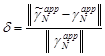
It seems crucial to analyze the highest order reconstruction provided by the
algorithm in case the errors accumulated from iteration to iteration. Figure 4
presents the results of boundary identification from the noisy data. The
depicted approximate profiles of
obtained
from noisy data.
It seems crucial to analyze the highest order reconstruction provided by the
algorithm in case the errors accumulated from iteration to iteration. Figure 4
presents the results of boundary identification from the noisy data. The
depicted approximate profiles of ![]() are
those obtained for
are
those obtained for ![]() in Examples 1-2 and
in Examples 1-2 and ![]() in Example 3.
in Example 3.
|
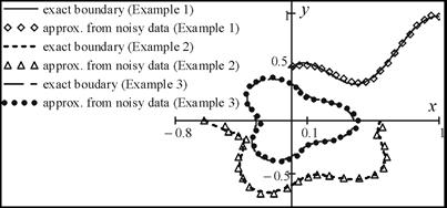
Fig. 4. Results of boundary identification from data containing 3% noise
Visual inspection of Figure 4 shows a fairly
good agreement between exact
and approximate positions of the corresponding boundary points. It indicates
small impact of the measurement errors on the predicted locations of the
unknown boundary points. In support of this conclusion, we present the errors (d ) between the
reconstructions of ![]() from clean and
noisy data (see Table 4).
from clean and
noisy data (see Table 4).
Table 4
Impact of 3% noise in the input data on boundary identification
|
|
Example 1 (N = 8) |
Example 2 (N = 8) |
Example 3 (N = 9) |
|
d [%] |
2.06 |
3.01 |
4.06 |
The percentage changes in boundary approximations - when compared to the measurement errors - are of the same order of magnitude. In conclusion, at the assumed level of noise, the algorithm turned out to be stable.
7. Conclusions and final remarks
We proposed an algorithm for identification of the unknown part of a domain boundary. Unlike the existing approaches based on the Trefftz method, the present algorithm offers a continuous solution which accurately recovers the unknown shape after a few iterations, as demonstrated in the included examples. Small random errors introduced to the input data resulted in comparably small disturbances in the final boundary reconstructions, which proved numerical stability of the solutions. Another advantage of the method is that it separates specification of the coefficients: those referring to temperature approximation are obtained from a linear system of equations while the coefficients of a shape approximation - from a distinct nonlinear system of equations with relatively few unknowns. That way, large (and numerically problematic) systems of nonlinear equations can be avoided. Finally, the proposed method can be extended without changes on boundary identification problems governed by other linear differential equations for which the T-complete functions are known or can be somehow generated.
References
[1] Marin L., Karageorghis A., Regularized MFS-based boundary identification in two-dimensional Helmholtz-type equation, CMC: Computers, Materials & Continua 2008, 10, 3, 259-293.
[2] Gonzalez M., Goldschmit M., Inverse geometry heat transfer problem based on radial basis functions geometry representation, International Journal for Numerical Methods in Engineering 2006, 65, 8, 1243-1268.
[3] Lesnic D., Berger J.R., Martin P.A., A boundary element regularization method for the boundary determination in potential corrosion damage, Inverse Problems in Engineering 2002, 10, 2, 163-182.
[4] Kazemzadeh-Parsi M.J., Daneshmand F., Solution of geometric inverse conduction problems by smoothed fixed grid finite element method, Finite Elements in Analysis and Design 2009, 45, 599-611.
[5] Burger M., A framework for the construction of level set methods for shape optimization and reconstruction, Interfaces and Free Boundaries 2003, 5, 301-329.
[6] Fan C.-M., Chan H.-F., Modified collocation Trefftz method for the geometry boundary identification problem of heat conduction, Numerical Heat Transfer, Part B 2011, 59, 58-75.
[7] Fan C.-M., Chan H.-F., Kuo C.-L., Yeih W., Numerical solutions of boundary detection problems using modified collocation Trefftz method and exponentially convergent scalar homotopy algorithm, Engineering Analysis with Boundary Elements 2012, 36, 2-8.
[8] Chan H.-F., Fan C.-M., The modified collocation Trefftz method and exponentially convergent scalar homotopy algorithm for the inverse boundary determination problem for the biharmonic equation, Journal of Mechanics 2013, 29, 02, 363-372.
[9] Fan C.-M., Liu Y.-C., Chan H.-F., Hsiao S.-S., Solutions of boundary detection problems for modified Helmholz equation by Trefftz method, Inverse Problems in Science and Engineering 2014, 22, 2, 267-281.
[10] Karageorghis A., Lesnic D., Marin L., Regularized collocation Trefftz method for void detection in two-dimensional steady-state heat conduction problems, Inverse Problems in Science and Engineering 2014, 22, 3, 395-418.
[11] Marin L., Karageorghis A., Lesnic D., The MFS for numerical boundary identification in two-dimensional harmonic problems, Engineering Analysis with Boundary Elements 2011, 35, 342-354.
[12] Karageorghis A., Lesnic D., Marin L., The MFS for inverse geometric problems, [in:] Inverse Problems and Computational Mechanics, eds. L. Marin, L. Munteanu, V. Chiroiu, Editura Academiei Române, Bucharest 2011.