Boundary integral solution for a class of fourth-order two-point boundary value problems

• BibTex
• RIS
• APA
• Harvard
• IEEE
• MLA
• Vancouver
• Chicago

@article{Al-Gahtani_2016,
   doi = {10.17512/jamcm.2016.3.01},
   url = {https://doi.org/10.17512/jamcm.2016.3.01},
   year = 2016,
   publisher = {The Publishing Office of Czestochowa University of Technology},
   volume = {15},
   number = {3},
   pages = {5--13},
   author = {Husain J. Al-Gahtani},
   title = {Boundary integral solution for a class of fourth-order two-point boundary value problems},
   journal = {Journal of Applied Mathematics and Computational Mechanics}
}

TY  - JOUR
DO  - 10.17512/jamcm.2016.3.01
UR  - https://doi.org/10.17512/jamcm.2016.3.01
TI  - Boundary integral solution for a class of fourth-order two-point boundary value problems
T2  - Journal of Applied Mathematics and Computational Mechanics
JA  - J Appl Math Comput Mech
AU  - Al-Gahtani, Husain J.
PY  - 2016
PB  - The Publishing Office of Czestochowa University of Technology
SP  - 5
EP  - 13
IS  - 3
VL  - 15
SN  - 2299-9965
SN  - 2353-0588
ER  - 

Al-Gahtani, H. (2016). Boundary integral solution for a class of fourth-order two-point boundary value problems. Journal of Applied Mathematics and Computational Mechanics, 15(3), 5-13. doi:10.17512/jamcm.2016.3.01

Al-Gahtani, H., 2016. Boundary integral solution for a class of fourth-order two-point boundary value problems. Journal of Applied Mathematics and Computational Mechanics, 15(3), pp.5-13. Available at: https://doi.org/10.17512/jamcm.2016.3.01

[1]H. Al-Gahtani, "Boundary integral solution for a class of fourth-order two-point boundary value problems," Journal of Applied Mathematics and Computational Mechanics, vol. 15, no. 3, pp. 5-13, 2016.

Al-Gahtani, Husain J.. "Boundary integral solution for a class of fourth-order two-point boundary value problems." Journal of Applied Mathematics and Computational Mechanics 15.3 (2016): 5-13. CrossRef. Web.

1. Al-Gahtani H. Boundary integral solution for a class of fourth-order two-point boundary value problems. Journal of Applied Mathematics and Computational Mechanics. The Publishing Office of Czestochowa University of Technology; 2016;15(3):5-13. Available from: https://doi.org/10.17512/jamcm.2016.3.01

Al-Gahtani, Husain J.. "Boundary integral solution for a class of fourth-order two-point boundary value problems." Journal of Applied Mathematics and Computational Mechanics 15, no. 3 (2016): 5-13. doi:10.17512/jamcm.2016.3.01

BOUNDARY INTEGRAL SOLUTION FOR A CLASS OF FOURTH-ORDER TWO-POINT BOUNDARY VALUE PROBLEMS

Husain J. Al-Gahtani

King Fahd University of Petroleum & Minerals
Dhahran, Saudi Arabia
hqahtani@kfupm.edu.sa

Abstract. In this paper, a boundary integral method is proposed for the solution of a class of fourth-order two-boundary value problems described by the equation , where P is a polynomial function of its arguments. The differential equation is cast in an integral form and the weighted residual technique is used to generate the corresponding boundary integral equations. The boundary integral equations are then, solved by expressing the dependent variable, y, in terms of a power series. The proposed method is tested through four examples to show the applicability of the method to solve a wide range of fourth-order differential equations including the nonlinear ones.

Keywords: boundary integral method, fourth-order differential equation, non-linear ordinary differential equations

1. Introduction

Many problems in applied science and engineering are modelled by fourth-order differential ordinary differential equations. Examples are bending of beams and axisymmetric shells, viscoelastic and inelastic flows, and electric circuits to mention a few. Classical methods for obtaining exact solutions are limited to certain types of linear equations with simple boundary conditions. Particularly in nonlinear ordinary differential equations, obtaining such solutions becomes difficult and sometimes impossible and therefore one has to resort to semi-analytical or numerical methods [1-4]. The objective of this paper is to present a boundary integral method [5-7] for solving a class of boundary value problems which are represented by fourth-order ordinary differential equations of the following form:

,

(1)

where P is a polynomial function of its arguments, and therefore the differential equation could be linear or nonlinear depending on the form of P.

The proposed method consists of two steps: First, Eq. (1) is cast in an integral form (Eqs. (8), (9) and (10)). Then, the integral equations (8), (9) and (10) are solved by expressing the dependent variable y as a power series, the coefficients of which can be obtained by equating the terms of similar powers. In the next section, the integral equations are derived for general fourth order boundary value problems. This is followed by a brief description of procedure for generating the power series solution. Finally, the method’s capabilities are demonstrated through numerical examples.

2. Integral equations

The boundary and domain integral equations corresponding to Eq. (1) can be obtained by multiplying both sides of Eq. (1) by a weighing function y* and integrating by parts four times over the domain (0,L), to get

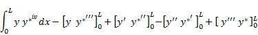
(2)

In order to get rid of the first domain integral, let us choose y* to be the fundamental solution corresponding to the fourth order operator, i.e. y* satisfies the following equation:

,

(3)

where is Dirac delta function, which has the following properties:

(4)

(5)

Using Eq. (3) in Eq. (2), we get the following equation

(6)

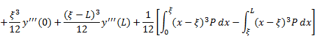
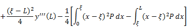
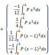
Once, the weighing function is obtained, Eq. (6) yields the solution y in terms of the boundary terms and the integral containing P. can be obtained by successive integration of (3):

	(7a)
	(7b)
	(7c)
	(7d)

where for and for . Using Eq. (7a) to (7d) in Eq. (6), we get

(8)

The first derivative of the solution can be obtained by differentiating Eq. (8) with respect to ξ

(9)

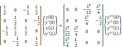
Similarly, higher order derivatives can be obtained by taking the proper derivatives of Eq. (8). Equations (8) and (9) provide the solution and its derivative at any domain point in terms of the boundary values and the forcing function P and therefore, called the domain integral equations. In order to generate four equations necessary for obtaining the unknown boundary values in terms of the known boundary conditions, Eqs. (8) and (9) need to be applied at the two boundary points and . The resulted equations, written in a matrix form, are:

(10)

In a well-posed problem, half of the boundary values are known and therefore, if the polynomial P happened to be a function of x only, the above four equations can be used directly to obtain the other non-specified boundary values which in turn can be used in Eq. (8) to obtain the exact solution for the problem. On the other hand, If P happens to be a function of y and/or its derivatives, then the solution procedure proposed in the following section can be implemented.

3. Solution of the integral equations

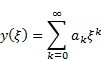
First, we represent the solution y(ξ) by a power series, i.e.

(11)

Inserting Eq. (11) into the right-hand side of Eq. (10) will transform the difficult integrals on the right-hand side of Eq. (10) into more readily solvable integrals and therefore the equation can be solved for the remaining boundary values in terms of the coefficients a_k. In order to obtain the coefficients a_k, k ≥ 0, use Eq. (11) and the results obtained from Eq. (10) in Eq. (8) and compute the integrals term by term to obtain an equation of the following form:

(12)

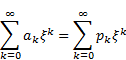
where p_k is a polynomial in a_k the form of which depends on the form of P that we started with. Equating the coefficients of similar powers of ξ from both sides, i.e. a_k = p_k leads to the complete determination of the coefficients a_k , k ≥ 0, hence obtaining the required solution of Eq. (1). It should be noted that if P is nonlinear, p_k will also be nonlinear and therefore the determination of the coefficients a_k will involve solving nonlinear algebraic equations. To check the efficeincy of the proposed method, four examples are given below.

4. Numerical examples

To illustrate the implementation of the proposed method, we consider the following four examples. For comparison reasons, the problems have homogenous and nonhomogeneous boundary conditions and known solutions. All symbolic computations are performed using Mathematica.

Example 1. For the purpose of explaining the procedure of the method in detail, we will start with the following fourth order differential equation with constant coefficients

(13)

subject to the following boundary conditions:, , and , which has the exact solution:

(14)

Inserting y as expressed by Eq. (11) and the above four boundary conditions in Eq. (10) with P = and L = 1, we get the four non-prescribed boundary variables

	(15)
	(16)
	(17)
	(18)

Using Eqs. (15)-(18), along with the given boundary conditions and the power series expansion of y in Eq. (8) and collecting coefficients of similar powers of ξ, yield the following equation

(19)

Equating the coefficients of similar powers of ξ, we obtain , , , , , , , hence is the exact solution of the problem is obtained.

Example 2. Consider the following fourth order differential equation with variable coefficients

,

(20)

subject to the boundary conditions The exact solution given by

(21)

Following the same procedure, we use Eq. (10) to solve for the four unknown boundary variables:

	(22)
	(23)
	(24)
	(25)

For n = 5, the process of using Eqs. (22)-(25) in Eq. (8) and equating coefficients of similar terms yields the solution for the first six coefficients: , , , , and , which is identical to the expansion of the exact solution given by Eq. (21). More terms can be obtained by increasing the order of the employed power series.

Example 3. Consider the following boundary value problem involving nonlinear boundary conditions which appears in the study of deformations of elastic beams on elastic bearings [8, 9]:

(26)

subject to the boundary conditions: , , , and . The appearance of third-order nonlinear boundary condition makes the problem challenging and difficult to solve. The exact solution of the above problem is given by [9]:

(27)

Following the same procedure and omitting the details, we obtain:

(28)

Equating the coefficients of similar powers of , we obtain: and .

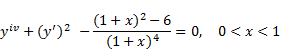
Example 4. In order to demonstrate the applicability of the method for solving nonlinear ordinary differential equations, let us consider the following one:

(29)

subject to the boundary conditions: , , , . The exact solution is given by [10]

(30)

Unlike the previous problems, the procedure of this one requires more power series terms in order to converge to the exact expansion of the solution given by Eq. (30). The convergence of the numerical values of the power series coefficients to their exact values is given in Table 1.

Table 1

Coefficients of power series solution

5. Conclusions

The numerical results confirm that the proposed boundary integral method is capable of obtaining an accurate power series solution to a wide class of boundary value problems represented by fourth order ordinary differential equations. The last two examples clearly indicate that the proposed method is accurate even with problems involving nonlinear differential equations and/or boundary conditions. Furthermore, the method is easy to program using any symbolic software.

Acknowledgements

The author would like to express his appreciation to King Fahd University of Petroleum & Minerals for supporting this study.

References

[1] Atkinson K., Han W., Stewart D., Numerical Solution of Ordinary Differential Equations, John Wiley, 2009.

[2] Butcher J., The Numerical Analysis of Ordinary Differential Equations: Runge-Kutta and General Linear Methods, John Wiley, 1987.

[3] Butcher J., The Numerical Methods for Ordinary Differential Equations: Runge-Kutta and General Linear Methods, John Wiley, 2003.

[4] LeVeque R., Finite difference methods for ordinary and partial differential equations, SIAM, 2007.

[5] Banerjee P., Butterheld R., Boundary Element Methods in Engineering Science, McGraw-Hill, London 1981.

[6] Butterfield R., New concepts illustrated by old problems, In: P.K. Banerjee, R. Butterfield (ed.), Development in Boundary Element Methods, London 1982.

[7] Al-Gahtani H., Integral-based solution for a class of second order boundary value problems, Applied Mathematics and Computation 1999, 98, 43-48.

[8] Ma T., Silva J., Iterative solutions for a beam equation with nonlinear boundary conditions of third order, Applied Mathematics and Computation 2004, 159, 11-18.

[9] Geng F., Iterative reproducing kernel method for a beam equation with third-order nonlinear boundary conditions. Mathematical Sciences 2012, 6-1, 1-4.

[10] El-Gamel M., Behiry S., Hashish H., Numerical method for the solution of special nonlinear fourth-order boundary value problems, Applied Mathematics and Computation 2004, 159, 11-18.