Steady-state characteristics of three-channel queueing systems with Erlangian service times
Bohdan Kopytko
,Kostyantyn Zhernovyi
Journal of Applied Mathematics and Computational Mechanics |
 Download Full Text |
 View in HTML format |
 Export citation |
@article{Kopytko_2016,
   doi = {10.17512/jamcm.2016.3.08},
   url = {https://doi.org/10.17512/jamcm.2016.3.08},
   year = 2016,
   publisher = {The Publishing Office of Czestochowa University of Technology},
   volume = {15},
   number = {3},
   pages = {75--87},
   author = {Bohdan Kopytko and  Kostyantyn Zhernovyi},
   title = {Steady-state characteristics of three-channel queueing systems with Erlangian service times},
   journal = {Journal of Applied Mathematics and Computational Mechanics}
}
TY - JOUR DO - 10.17512/jamcm.2016.3.08 UR - https://doi.org/10.17512/jamcm.2016.3.08 TI - Steady-state characteristics of three-channel queueing systems with Erlangian service times T2 - Journal of Applied Mathematics and Computational Mechanics JA - J Appl Math Comput Mech AU - Kopytko, Bohdan AU - Zhernovyi, Kostyantyn PY - 2016 PB - The Publishing Office of Czestochowa University of Technology SP - 75 EP - 87 IS - 3 VL - 15 SN - 2299-9965 SN - 2353-0588 ER -
Kopytko, B., & Zhernovyi, K. (2016). Steady-state characteristics of three-channel queueing systems with Erlangian service times. Journal of Applied Mathematics and Computational Mechanics, 15(3), 75-87. doi:10.17512/jamcm.2016.3.08
Kopytko, B. & Zhernovyi, K., 2016. Steady-state characteristics of three-channel queueing systems with Erlangian service times. Journal of Applied Mathematics and Computational Mechanics, 15(3), pp.75-87. Available at: https://doi.org/10.17512/jamcm.2016.3.08
[1]B. Kopytko and K. Zhernovyi, "Steady-state characteristics of three-channel queueing systems with Erlangian service times," Journal of Applied Mathematics and Computational Mechanics, vol. 15, no. 3, pp. 75-87, 2016.
Kopytko, Bohdan, and Kostyantyn Zhernovyi. "Steady-state characteristics of three-channel queueing systems with Erlangian service times." Journal of Applied Mathematics and Computational Mechanics 15.3 (2016): 75-87. CrossRef. Web.
1. Kopytko B, Zhernovyi K. Steady-state characteristics of three-channel queueing systems with Erlangian service times. Journal of Applied Mathematics and Computational Mechanics. The Publishing Office of Czestochowa University of Technology; 2016;15(3):75-87. Available from: https://doi.org/10.17512/jamcm.2016.3.08
Kopytko, Bohdan, and Kostyantyn Zhernovyi. "Steady-state characteristics of three-channel queueing systems with Erlangian service times." Journal of Applied Mathematics and Computational Mechanics 15, no. 3 (2016): 75-87. doi:10.17512/jamcm.2016.3.08
STEADY-STATE CHARACTERISTICS OF THREE-CHANNEL QUEUEING SYSTEMS WITH ERLANGIAN SERVICE TIMES
Bohdan Kopytko 1, Kostyantyn Zhernovyi 2
1 Institute of Mathematics,
Czestochowa University of Technology
Częstochowa, Poland
2 Educational and Scientific
Institute, Banking University
Lviv, Ukraine
bohdan.kopytko@im.pcz.pl, k.zhernovyi@yahoo.com
Abstract. We propose a method of study the M/E2/3/∞ queueing systems: standard system and systems with the threshold and hysteretic strategies of the random dropping of customers in order to control the input flow. Recurrence relations to compute the stationary distribution of the number of customers and the steady-state characteristics are obtained. The developed algorithms are tested on examples using simulation models constructed with the assistance of the GPSS World tools.
Keywords: three-channel queueing system, Poisson input, Erlangian service times, random dropping of customers, fictitious phase method, recurrence relations
1. Introduction
There are currently no created analytical
methods of study of the M/G/n/m
and M/G/n/∞ queueing systems with the number of channels ![]() The M/D/n/∞ system is one of the
few exceptions. It is possible to obtain some of the characteristics associated
with the number of customers in the system [1].
The M/D/n/∞ system is one of the
few exceptions. It is possible to obtain some of the characteristics associated
with the number of customers in the system [1].
To investigate the single-channel systems
with Erlangian service times, in
particular the M/Es/1/∞ system [1], the method of fictitious
phases, developed by Erlang [2], was applied. The Erlangian service times of
the order ![]() means that each customer
runs sequentially
means that each customer
runs sequentially ![]() service phases, the duration
of which is distributed exponentially
with parameters
service phases, the duration
of which is distributed exponentially
with parameters ![]() respectively.
respectively.
The objective of this work is the construction with the help of the method of fictitious phase recurrence algorithms for computing the stationary distribution of the number of customers in the three-channel queueing system M/E2/3/∞, as well as in the systems of the same type with threshold and hysteretic strategies of the random dropping of customers. The random dropping of arrivals is a powerful tool for parameter control of a queueing system. Each arriving customer can be accepted for service with a probability depending on the queue length at the time of arrival of the customer, even if the buffer is not completely full [3-6].
2. The M/E2/3/∞ system
We consider the
M/E2/3/∞ system. Let ![]() be a
parameter of the exponential distribution of the time intervals between moments
of arrival of customers. Suppose that the service time of each customer is
distributed under the generalized Erlang law of the second order, that is, the
service time is the sum of two independent
random variables exponentially
distributed with parameters
be a
parameter of the exponential distribution of the time intervals between moments
of arrival of customers. Suppose that the service time of each customer is
distributed under the generalized Erlang law of the second order, that is, the
service time is the sum of two independent
random variables exponentially
distributed with parameters ![]() and
and ![]() respectively.
respectively.
Let ![]() denote
the number of customers in the system and let
denote
the number of customers in the system and let ![]() be
the number of busy channels. In accordance with the method of phases, let us
enumerate the system’s states as follows:
be
the number of busy channels. In accordance with the method of phases, let us
enumerate the system’s states as follows: ![]() corresponds
to the empty system;
corresponds
to the empty system; ![]() is the state, when
is the state, when ![]() and the service occurs in the first
phase;
and the service occurs in the first
phase; ![]() is the state, when
is the state, when ![]() and the service occurs in the second
phase;
and the service occurs in the second
phase; ![]() is the state, when
is the state, when ![]() and the services occur in the first
phase;
and the services occur in the first
phase; ![]() is the state, when
is the state, when ![]() and the services occur in the first and
second phase respectively;
and the services occur in the first and
second phase respectively; ![]() is the state, when
is the state, when ![]() and the services occur in the second
phase;
and the services occur in the second
phase; ![]() is the state, when
is the state, when ![]() and the services occur in the first
phase;
and the services occur in the first
phase; ![]() is the state, when
is the state, when ![]() and the services in two channels
occur in the first phase and in one channel the service occurs in the second
phase;
and the services in two channels
occur in the first phase and in one channel the service occurs in the second
phase; ![]() is the state, when
is the state, when ![]() and the service in two channels
occur in the second phase and in one channel the service occurs in the first
phase;
and the service in two channels
occur in the second phase and in one channel the service occurs in the first
phase; ![]() is the state, when
is the state, when ![]() and the service occurs in the second
phase. We denote by
and the service occurs in the second
phase. We denote by ![]() and
and ![]()
![]() respectively, steady-state
probabilities that the system is in the each of these states. Assuming that
respectively, steady-state
probabilities that the system is in the each of these states. Assuming that ![]() to calculate the steady-state
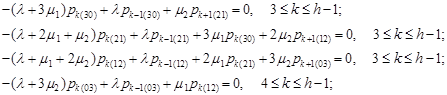
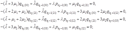
probabilities, we obtain the system of equations:
to calculate the steady-state
probabilities, we obtain the system of equations:
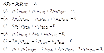 | (1) |
 | (2) |
| (3) |
The steady-state distribution of the number of customers in the M/E2/3/∞
system exists under the condition that ![]() where
where ![]() is the average service time
per customer.
is the average service time
per customer.
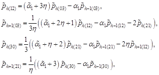
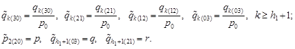
Introducing the notation
 |
| using equations (1) we find: |
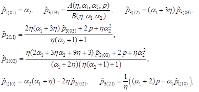 | (4) |
where
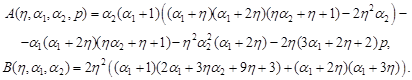 |
Recurrence
relations (4) contain the parameter ![]() to be determined.
to be determined.
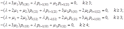
From equations (2) we obtain the recurrence relations:
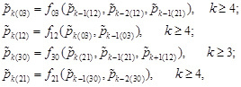 | (5) |
where
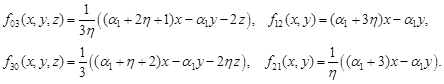 |
The system (1)-(3) consists of an infinite
number of equations. Let ![]() be a sufficiently
large natural number. Writing the normalization condition (3) in the form
be a sufficiently
large natural number. Writing the normalization condition (3) in the form
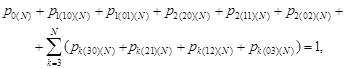 | (6) |
we determine the approximate values of the stationary probabilities using equations
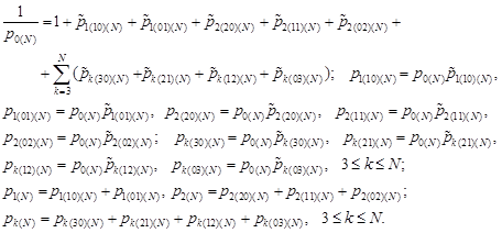 | (7) |
Here ![]() is the steady-state
probability that
is the steady-state
probability that ![]()
![]() is
the approximate value of the probability
is
the approximate value of the probability ![]() obtained
after replacing condition (3) by equality (6).
obtained
after replacing condition (3) by equality (6).
Recurrence
relations (4) and (5) allow us to calculate ![]() and consistently
obtain the expression for
and consistently
obtain the expression for ![]() and
and ![]()
![]() as functions of the unknown parameter
as functions of the unknown parameter ![]() To determine
To determine ![]() we use the condition that in
the steady state, the average number of busy channels is equal to the system load factor
we use the condition that in
the steady state, the average number of busy channels is equal to the system load factor ![]() writing it in the form
writing it in the form
Using the formulas
we find approximate values of the average queue
length ![]() and the average waiting time
and the average waiting time ![]() in the steady state. The number
in the steady state. The number ![]() is chosen so large that
the condition
is chosen so large that
the condition
| (8) |
holds, where ![]() is a positive number specifying
the required accuracy of calculations.
is a positive number specifying
the required accuracy of calculations.
3. The M/E2/3/∞ system with the threshold strategy of the random dropping of customers
We consider for the M/E2/3/∞
system a strategy of random dropping of customers performed according to the
rule: if at the time of the arrival of a customer ![]() (not
taking into account the arrived customer), then the customer is accepted for
service with probability
(not
taking into account the arrived customer), then the customer is accepted for
service with probability ![]() and leaves the
system (is discarded) with probability
and leaves the
system (is discarded) with probability ![]() Confining
ourselves to a simplified version of the strategy, let’s fix a threshold value
Confining
ourselves to a simplified version of the strategy, let’s fix a threshold value ![]() and suppose that
and suppose that ![]() for
for ![]() and
and ![]() for
for ![]() The
intensity of the simplest flow of customers
received for service as a result of random dropping, is equal to
The
intensity of the simplest flow of customers
received for service as a result of random dropping, is equal to ![]()
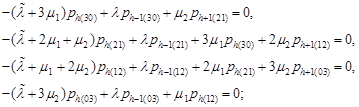
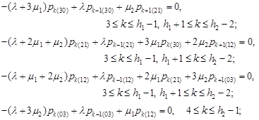
The system of equations for determining the steady-state probabilities contains the equation (1), (3) and the following equations:
 | (9) |
 | (10) |
 | (11) |
Using equations (1), we have the equalities (4) and from the equations (9) we obtain the recurrence relations:
 | (12) |
Using equation (10), we find:
 | (13) |
where ![]() From equations (11)
we obtain:
From equations (11)
we obtain:
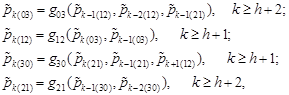 | (14) |
where
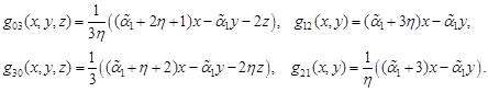 |
Recurrence
relations (4), (12)-(14) allow us to calculate ![]() and consistently obtain the expression for
and consistently obtain the expression for ![]() and
and ![]() as functions of the unknown parameter
as functions of the unknown parameter ![]() To
determine
To
determine ![]() we use the
condition that in the steady state the average number of busy channels
is equal
to the system load factor
we use the
condition that in the steady state the average number of busy channels
is equal
to the system load factor ![]() The steady-state probabilities exist under the condition that
The steady-state probabilities exist under the condition that ![]() We find the approximate values of
steady-state probabilities by the formulas (7) where
the number
We find the approximate values of
steady-state probabilities by the formulas (7) where
the number ![]() is chosen so large
that the condition (8) holds.
is chosen so large
that the condition (8) holds.
The approximate values of the average queue
length ![]() average waiting time
average waiting time ![]() and probability of service
and probability of service ![]() in the steady state
in the steady state
Using the formulas
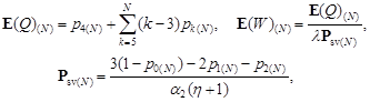 | (15) |
we find the approximate values of the average
queue length ![]() average waiting time
average waiting time ![]() and probability of service
and probability of service ![]() in the steady state. The formula for
in the steady state. The formula for ![]() is obtained as the ratio of the average
number of serviced customers per unit of time to the average arrival rate of
customers.
is obtained as the ratio of the average
number of serviced customers per unit of time to the average arrival rate of
customers.
4. The M/E2/3/∞ system with the hysteretic strategy of the random dropping of customers
We consider for
the M/E2/3/∞ system a hysteretic strategy of a random dropping of customers with two
thresholds ![]() and
and ![]() (
(![]() ) and with two operation modes: basic mode and
dropping mode. Assume that
) and with two operation modes: basic mode and
dropping mode. Assume that ![]() for the basic mode, and
for the basic mode, and ![]() for the dropping mode. Here
for the dropping mode. Here ![]() is the number of customers in the
system at the time of the arrival of a customer (not taking into account the
arrived customer). If at the time of the arrival of
a customer, condition
is the number of customers in the
system at the time of the arrival of a customer (not taking into account the
arrived customer). If at the time of the arrival of
a customer, condition ![]() is
satisfied, then the mode is not changed.
The dropping mode operates from the time when the number of customers in
the system (on service and in the
queue) reaches the value of
is
satisfied, then the mode is not changed.
The dropping mode operates from the time when the number of customers in
the system (on service and in the
queue) reaches the value of ![]() to the time when the number of
customers decreases to
to the time when the number of
customers decreases to ![]()
We introduce the following notation for the states of the system in the basic mode: the states ![]() correspond to the notation introduced
above,
correspond to the notation introduced
above, ![]() is the state,
when
is the state,
when ![]() and the services occur in the first
phase;
and the services occur in the first
phase; ![]() is the state, when
is the state, when ![]() and the services in
two channels occur in the first phase and in one channel the service occurs in
the second phase;
and the services in
two channels occur in the first phase and in one channel the service occurs in
the second phase; ![]() is the state, when
is the state, when ![]() and the service in
two channels occur in the second phase and in one channel the service occurs in the first phase;
and the service in
two channels occur in the second phase and in one channel the service occurs in the first phase; ![]() is the state, when
is the state, when ![]() and the service occurs in the second phase. We denote by
and the service occurs in the second phase. We denote by ![]()
![]() and
and ![]()
![]() respectively, the steady-state probabilities that the system is in
each of mentioned states. We denote by
respectively, the steady-state probabilities that the system is in
each of mentioned states. We denote by ![]() and
and ![]() analogous states of the
system in the dropping mode and let
analogous states of the
system in the dropping mode and let ![]() and
and ![]()
![]() denote
the steady-state probabilities that the system is in
each of these states.
denote
the steady-state probabilities that the system is in
each of these states.
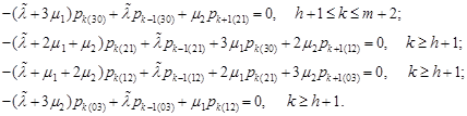
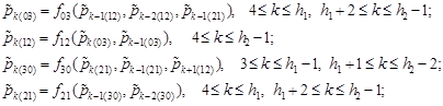
For determining the steady-state probabilities, we obtain the system containing the equation (1) and the following equations:
 | (16) |
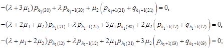 | (17) |
| (18) |
| (19) |
| (20) |
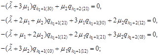 | (21) |
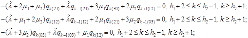 | (22) |
 | (23) |
 | (24) |
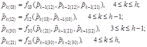
Introduce the notation
 |
Using equations (1), we have the equalities (4) and from the equations (16) we obtain the recurrence relations:
 | (25) |
Using equations (17), (21), (22) and (18), we find:
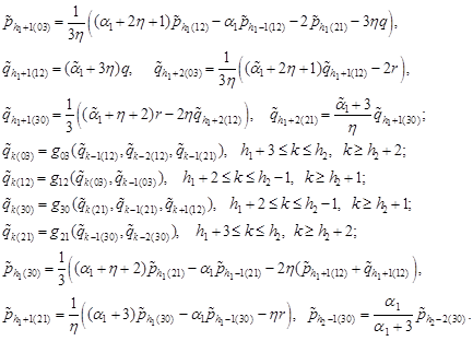 | (26) |
To determine ![]() and
and ![]() as functions of the parameter
as functions of the parameter ![]() we use the equations (19) and
(20).
we use the equations (19) and
(20).
The equations (23) allow us to find
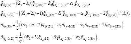 | (27) |
To determine ![]() we use the condition that in the
steady state the average number of busy channels is equal
to the system load factor
we use the condition that in the
steady state the average number of busy channels is equal
to the system load factor
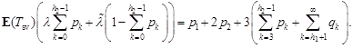 |
The steady-state probabilities exist under
the condition that ![]() Using the recurrence
relations (25)-(27) and the normalization condition (24), we obtain the
approximate values of the steady-state probabilities from the equalities:
Using the recurrence
relations (25)-(27) and the normalization condition (24), we obtain the
approximate values of the steady-state probabilities from the equalities:
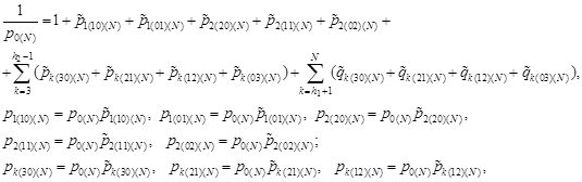 |
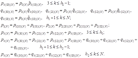 |
Using the formulas
(15) we find the approximate values of the stationary characteristics ![]() and
and ![]()
5. Examples for the calculating of stationary characteristics
Introduce the notation for the studied queueing systems. Let the M/E2/3/∞ system be the System 1, the M/E2/3/∞ system with the threshold strategy of the random dropping of customers be the System 2 and the M/E2/3/∞ system with the hysteretic strategy of the random dropping of customers be the System 3.
For all
the systems we put: ![]() Let
Let ![]() for the System 1,
for the System 1, ![]() for the Systems 2 and 3,
for the Systems 2 and 3, ![]() for the System 2,
for the System 2, ![]() for the System 3.
for the System 3.
The values of the steady-state probabilities
and stationary characteristics of
the systems 1-3, found using the recurrence relations obtained in this paper,
are presented in Tables 1 and 2. In order to verify the obtained values,
the tables
contain the computing results evaluated by the GPSS World simulation system [7]
for the time value ![]()
In
calculating the approximate values of the steady-state probabilities ![]() the number
the number ![]() is chosen so large
that the condition
is chosen so large
that the condition
| (28) |
holds. The obtained minimum values of ![]() for which the condition (28) is satisfied, are
equal to 156, 164 and 162 for the Systems 1, 2 and 3, respectively.
for which the condition (28) is satisfied, are
equal to 156, 164 and 162 for the Systems 1, 2 and 3, respectively.
Table 1
Stationary distribution of the number of customers in the system (1 - analytical method, 2 - GPSS World)
|
k |
Values of the steady-state probabilities pk |
|||||
|
System 1 |
System 2 |
System 3 |
||||
|
1, N = 156 |
2 |
1, N = 164 |
2 |
1, N = 162 |
2 |
|
|
0 |
0.0241532 |
0.0241463 |
0.0019693 |
0.0019621 |
0.0028508 |
0.0028780 |
|
1 |
0.0666245 |
0.0664944 |
0.0068771 |
0.0068758 |
0.0099553 |
0.0100608 |
|
2 |
0.0942915 |
0.0942690 |
0.0124350 |
0.0124441 |
0.0180009 |
0.0180814 |
|
3 |
0.0954951 |
0.0954166 |
0.0163353 |
0.0163913 |
0.0236470 |
0.0237228 |
|
4 |
0.0881153 |
0.0881351 |
0.0197881 |
0.0198060 |
0.0286452 |
0.0287503 |
|
5 |
0.0786458 |
0.0785520 |
0.0233579 |
0.0233281 |
0.0338128 |
0.0338232 |
|
6 |
0.0693057 |
0.0694374 |
0.0273314 |
0.0272895 |
0.0395640 |
0.0395121 |
|
7 |
0.0607719 |
0.0609322 |
0.0318850 |
0.0317958 |
0.0461397 |
0.0460776 |
|
8 |
0.0531851 |
0.0530799 |
0.0371591 |
0.0368896 |
0.0536338 |
0.0536840 |
|
9 |
0.0465099 |
0.0465122 |
0.0432901 |
0.0432911 |
0.0618105 |
0.0619795 |
|
10 |
0.0406604 |
0.0405606 |
0.0504217 |
0.0503929 |
0.0667520 |
0.0670598 |
|
20 |
0.0105844 |
0.0105622 |
0.0296765 |
0.0297640 |
0.0236203 |
0.0235319 |
|
30 |
0.0027549 |
0.0027422 |
0.0077243 |
0.0078382 |
0.0061479 |
0.0060459 |
|
40 |
0.0007170 |
0.0007173 |
0.0020105 |
0.0019613 |
0.0016002 |
0.0016040 |
|
50 |
0.0001866 |
0.0002080 |
0.0005233 |
0.0005068 |
0.0004165 |
0.0004464 |
|
60 |
0.0000486 |
0.0000583 |
0.0001362 |
0.0001378 |
0.0001084 |
0.0001119 |
|
70 |
0.0000126 |
0.0000162 |
0.0000355 |
0.0000264 |
0.0000282 |
0.0000277 |
|
80 |
0.0000033 |
0.0000062 |
0.0000092 |
0.0000095 |
0.0000073 |
0.0000074 |
|
90 |
8.566∙10–7 |
0.0000008 |
0.0000024 |
0.0000014 |
0.0000019 |
0.0000011 |
|
100 |
2.229∙10–7 |
0.0000008 |
6.251∙10–7 |
0.0000013 |
4.975∙10–7 |
0.0000002 |
|
110 |
5.803∙10–8 |
0.0000000 |
1.626∙10–7 |
0.0000009 |
1.295∙10–7 |
0.0000000 |
|
130 |
3.931∙10–9 |
|
1.102∙10–8 |
0.0000000 |
8.773∙10–9 |
|
|
150 |
2.663∙10–10 |
|
7.467∙10–10 |
|
5.943∙10–10 |
|
Table 2
Stationary characteristics of the system
|
The system number |
Method |
E(Q) |
E(W) |
Psv |
|
1 |
analytical |
5.7429114 |
3.1905063 |
1 |
|
1 |
GPSS World |
5.745 |
3.193 |
1 |
|
2 |
analytical |
12.3769008 |
6.2553772 |
0.8793786 |
|
2 |
GPSS World |
12.378 |
6.256 |
0.879 |
|
3 |
analytical |
10.7951977 |
5.4825119 |
0.8751218 |
|
3 |
GPSS World |
10.790 |
5.478 |
0.875 |
6. Conclusions
The numerical algorithm for solving a system of linear algebraic equations for the steady-state probabilities, proposed in this paper, is constructed taking into account the structural features of the system, in particular the presence of three or four unknown in most of its equations. The obtained recurrence relations are used for the direct calculation of the solutions of the system, that allow us to reduce the number of calculations in comparison with application of one of the classical methods (direct or iterative). Direct methods require the implementation of preliminary transformations of the matrix of the system, and only in the second stage of computing the solutions is consistently defined. When using iterative methods, the calculations are performed repeatedly until a solution is found with a given accuracy. The use of iterative methods is possible only under the condition of diagonal dominance of the matrix of the system.
References
[1] Bocharov P.P., Pechinkin A.V., Queueing Theory, RUDN, Moskow 1995 (in Russian).
[2] Brockmeyer E., Halstrøm H.L., Jensen A., The Life and Works of A.K. Erlang, Danish Academy of Technical Sciences, Copenhagen 1948.
[3] Chydziński A., Nowe modele kolejkowe dla węzłów sieci pakietowych, Pracownia Komputerowa Jacka Skalmierskiego, Gliwice 2013 (in Polish).
[4] Tikhonenko O., Kempa W.M., Queue-size distribution in M/G/1-type system with bounded capacity and packet dropping, Communications in Computer and Information Science 2013, 356, 177-186.
[5] Zhernovyi Yu., Kopytko B., Zhernovyi K., On characteristics of the Mθ/G/1/m and Mθ/G/1 queues with queue-size based packet dropping, Journal of Applied Mathematics and Computational Mechanics 2014, 13(4), 163-175.
[6] Zhernovyi Yu.V., Zhernovyi K.Yu., Potentials method for M/G/1/m systems with threshold operating strategies, Cybernetics and Systems Analysis 2016, 52, 3, 481-491.
[7] Zhernovyi Yu., Creating Models of Queueing Systems Using GPSS World, LAP Lambert Academic Publishing, Saarbrücken 2015.
