Quartic non-polynomial spline solution for solving two-point boundary value problems by using Conjugate Gradient Iterative Method
Hynichearry Justine
,Jackel Vui Ling Chew
,Jumat Sulaiman
Journal of Applied Mathematics and Computational Mechanics |
 Download Full Text |
 View in HTML format |
 Export citation |
@article{Justine_2017,
   doi = {10.17512/jamcm.2017.1.04},
   url = {https://doi.org/10.17512/jamcm.2017.1.04},
   year = 2017,
   publisher = {The Publishing Office of Czestochowa University of Technology},
   volume = {16},
   number = {1},
   pages = {41--50},
   author = {Hynichearry Justine and  Jackel Vui Ling Chew and  Jumat Sulaiman},
   title = {Quartic non-polynomial spline solution for solving two-point boundary value problems by using Conjugate Gradient Iterative Method},
   journal = {Journal of Applied Mathematics and Computational Mechanics}
}
TY - JOUR DO - 10.17512/jamcm.2017.1.04 UR - https://doi.org/10.17512/jamcm.2017.1.04 TI - Quartic non-polynomial spline solution for solving two-point boundary value problems by using Conjugate Gradient Iterative Method T2 - Journal of Applied Mathematics and Computational Mechanics JA - J Appl Math Comput Mech AU - Justine, Hynichearry AU - Chew, Jackel Vui Ling AU - Sulaiman, Jumat PY - 2017 PB - The Publishing Office of Czestochowa University of Technology SP - 41 EP - 50 IS - 1 VL - 16 SN - 2299-9965 SN - 2353-0588 ER -
Justine, H., Chew, J., & Sulaiman, J. (2017). Quartic non-polynomial spline solution for solving two-point boundary value problems by using Conjugate Gradient Iterative Method. Journal of Applied Mathematics and Computational Mechanics, 16(1), 41-50. doi:10.17512/jamcm.2017.1.04
Justine, H., Chew, J. & Sulaiman, J., 2017. Quartic non-polynomial spline solution for solving two-point boundary value problems by using Conjugate Gradient Iterative Method. Journal of Applied Mathematics and Computational Mechanics, 16(1), pp.41-50. Available at: https://doi.org/10.17512/jamcm.2017.1.04
[1]H. Justine, J. Chew and J. Sulaiman, "Quartic non-polynomial spline solution for solving two-point boundary value problems by using Conjugate Gradient Iterative Method," Journal of Applied Mathematics and Computational Mechanics, vol. 16, no. 1, pp. 41-50, 2017.
Justine, Hynichearry, Jackel Vui Ling Chew, and Jumat Sulaiman. "Quartic non-polynomial spline solution for solving two-point boundary value problems by using Conjugate Gradient Iterative Method." Journal of Applied Mathematics and Computational Mechanics 16.1 (2017): 41-50. CrossRef. Web.
1. Justine H, Chew J, Sulaiman J. Quartic non-polynomial spline solution for solving two-point boundary value problems by using Conjugate Gradient Iterative Method. Journal of Applied Mathematics and Computational Mechanics. The Publishing Office of Czestochowa University of Technology; 2017;16(1):41-50. Available from: https://doi.org/10.17512/jamcm.2017.1.04
Justine, Hynichearry, Jackel Vui Ling Chew, and Jumat Sulaiman. "Quartic non-polynomial spline solution for solving two-point boundary value problems by using Conjugate Gradient Iterative Method." Journal of Applied Mathematics and Computational Mechanics 16, no. 1 (2017): 41-50. doi:10.17512/jamcm.2017.1.04
QUARTIC NON-POLYNOMIAL SPLINE SOLUTION FOR SOLVING TWO-POINT BOUNDARY VALUE PROBLEMS BY USING CONJUGATE GRADIENT ITERATIVE METHOD
Hynichearry Justine, Jackel Vui Ling Chew, Jumat Sulaiman
Mathematics with Economics Programme,
University Malaysia Sabah
Sabah, Malaysia
cherryjust20@gmail.com, jackelchew93@gmail.com, jumat@ums.edu.my
Received: 23 November 2016; accepted:
10 February 2017
Abstract. Solving two-point boundary value problems has become a scope of interest among many researchers due to its significant contributions in the field of science, engineering, and economics which is evidently apparent in many previous literary publications. This present paper aims to discretize the two-point boundary value problems by using a quartic non-polynomial spline before finally solving them iteratively with Conjugate Gradient (CG) method. Then, the performances of the proposed approach in terms of iteration number, execution time and maximum absolute error are compared with Gauss-Seidel (GS) and Successive Over-Relaxation (SOR) iterative methods. Based on the performances analysis, the two-point boundary value problems are found to have the most favorable results when solved using CG compared to GS and SOR methods.
MSC 2010: 34B05
Keywords: two-point boundary value problems, quartic non-polynomial spline, Conjugate Gradient, Successive Over-Relaxation, Gauss-Seidel
1. Introduction
Numerical methods have numerous significances in the field of sciences, economics, and engineering, and one of them when it comes to the solution of two-point boundary value problems which involve finding an approximate solution iteratively, as it will be time-consuming to solve them with analytical method. Some of the contributions of numerical methods related to the two-point boundary value problems include the modelling of chemical reactions and the modelling of heat transfer, such as in rocket thrust chamber liners and in the fuel elements for nuclear reactors as discussed by Ozisik [1]. On the other hand, Goffe [2] mentioned the modelling of the growth theory, capital theory, investment theory, resource economics and labor economics in the field of economics. Prior to these, many researchers had attempted to initiate different methods in order to accelerate the approximate solution when solving the problems and this can be abundantly found in previous literary publications. Some of the methods that were readily apparent are the Newton-EGMSOR method [3], the EADM method [4], the shooting method [5], the PTI method [6], the nonlinear shooting method [7], the mean weight method [8], the finite difference, the finite element and the finite volume method [9] and the spline method [10, 11]. Despite all these methods, the solution in this paper was given focus based on the discretization of the quartic non-polynomial spline together with the Conjugate Gradient (CG) iterative method.
Moreover, there are many other iterative methods which are thoroughly discussed by Kelly [12], Burgerscentrum [13], Hestenes and Stiefel [14], Saad [15], Hackbush [16] and Young [17, 18]. According to Ibrahim and Abdullah [19], and Yousif and Evans [20], there are several numbers of the iterative methods family with a different concept, and they emphasized the concept of block iteration. In addition to that, Ul-Islam et al. [21], Ramadan et al. [22], Siddiqi et al. [23] have provided the basis for this paper at a different degree of splines to solve the two-point boundary value problems. In regards to the advantages of the CG iterative method and the spline approach as highlighted in [14] and [21-23] respectively, this present paper aims to develop a solution for the problems by using a quartic non-polynomial spline together with the CG iterative method. As for comparison purposes, Successive Over-Relaxation (SOR) and Gauss-Seidel (GS) were set as control methods so that the performances of the CG method can be determined in respect to its iteration number, execution time and maximum absolute error.
2. Two-point boundary value problems
Generally, the two-point boundary value problems can be expressed as Eq. (1) and subject to boundary conditions (2) as follows:
| (1) |
| (2) |
where![]()
![]() and
and ![]() are
known functions restricted by boundary
are
known functions restricted by boundary ![]() and
and ![]()
![]() is
a constant. The solution for problem (1) cannot be obtained through
a random selection of functions
is
a constant. The solution for problem (1) cannot be obtained through
a random selection of functions![]()
![]() and
and ![]() due
to the restrictions held
by the boundary conditions (2). Furthermore, the process for discretization of
problem (1) is made simpler by assuming positive integer
due
to the restrictions held
by the boundary conditions (2). Furthermore, the process for discretization of
problem (1) is made simpler by assuming positive integer ![]()
![]() and
letting
the solution domain,
and
letting
the solution domain, ![]() be divided uniformly into a uniform separation of nodes set
or subinterval,
be divided uniformly into a uniform separation of nodes set
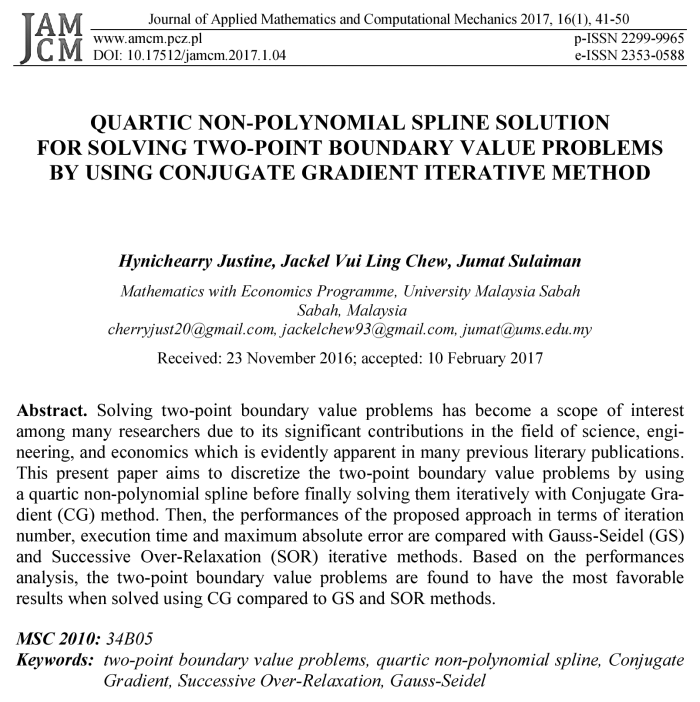
or subinterval, ![]() as shown in Figure 1.
Then, the length of the uniform
subintervals,
as shown in Figure 1.
Then, the length of the uniform
subintervals, ![]() can be defined as:
can be defined as:
| (3) |
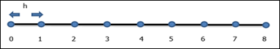
Fig. 1. Distribution of node point for domain solution m = 8
Moreover, the solution domain in Figure 1 was
used to develop a uniform grid
of a/the network as shown in Figure 2 for the derivation of the spline
function, and the grid points in the solution domain were labeled as ![]()
![]() with
function
with
function ![]() denoted as
denoted as ![]() The
formulation and implementation of the GS, SOR and CG iterative method were then
conducted based on the interior grid points until the convergence test is satisfied.
The
formulation and implementation of the GS, SOR and CG iterative method were then
conducted based on the interior grid points until the convergence test is satisfied.
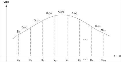
Fig. 2. Illustration of non-polynomial spline function for domain solution m = 8
3. Quartic non-polynomial spline approximation equation
The general form of the non-polynomial spline can be expressed as follows:
| (4) |
and it was used to discretize the problem (1) so
that the approximation equation can be constructed as a system of linear equations
in a matrix form. This discretization process was conducted by assuming ![]() as the exact solution for problem (1)
and
as the exact solution for problem (1)
and ![]() as the quartic non-polynomial spline
approximation to
as the quartic non-polynomial spline
approximation to ![]() obtained from the mixed
splines
obtained from the mixed
splines ![]() as shown in Figure 2 which passing
through the points
as shown in Figure 2 which passing
through the points ![]() and
and ![]() .
Based on Eq. (4), the quartic non-polynomial spline can be expressed in
.
Based on Eq. (4), the quartic non-polynomial spline can be expressed in ![]() as:
as:
| (5) |
where ![]() and
and ![]() are constants for
are constants for ![]() and
and ![]() is a
free parameter [19]. The function
is a
free parameter [19]. The function ![]() interpolates
interpolates ![]() at the points
at the points ![]() by
depending on
by
depending on ![]() and reducing to quartic spline in
and reducing to quartic spline in ![]() as
as ![]()
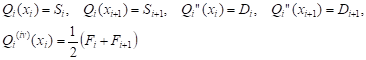
Then, in order to obtain the necessary
conditions for all the constants
![]() and,
and,![]() the
function
the
function ![]() has been satisfied at
has been satisfied at ![]() and
and ![]() at
boundary conditions (2) and at the continuity of the common nodes at
at
boundary conditions (2) and at the continuity of the common nodes at ![]() of first, second and third derivatives. Before deriving the
expression for all the coefficients of (6) in terms of
of first, second and third derivatives. Before deriving the
expression for all the coefficients of (6) in terms of ![]() and
and ![]() we first define the
function
we first define the
function ![]() at second and fourth derivatives as:
at second and fourth derivatives as:
 | (6) |
After performing a straightforward
calculation, all the values (7) of constant ![]() and,
and,
![]() were obtained as follows:
were obtained as follows:
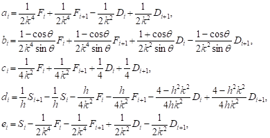 (7) (7) |
where ![]() and
and ![]()
Now that all the values of constant ![]() and,
and, ![]() were
obtained, we then use the continuity conditions (2) of the quartic spline
were
obtained, we then use the continuity conditions (2) of the quartic spline ![]() at its first and third derivatives at
the point
at its first and third derivatives at
the point ![]() where the two quartics
where the two quartics ![]() and
and ![]() join,
and this relation can be written as:
join,
and this relation can be written as:
where the degree of the derivative is ![]()
Based on Eqs. (5) and (7), the relation at the first derivative (8) and the third derivative (9) can be expressed in following form:
| (8) |
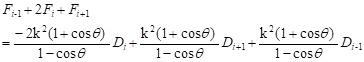 | (9) |
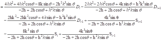
Upon subtraction of Eqs. (8) and (9), it yields the following equation:
|
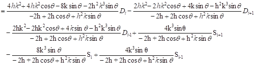
Then, a system of linear equations is constructed based on (10) in the following form:
| (11) |
where 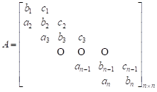
![]() and
and ![]()
4. Algorithm of CG method
The CG iterative method was first discussed
by Hestenes and Stiefel [14] as mentioned earlier, and this iterative method
will converge in less than or equal to the size of the matrix itself in the
absence of round-off error, with the assumption that matrix ![]() in (11) is symmetric and positive
definite. In fact, this method surpassed the Gauss elimination method. In
addition to that, the CG method is much simpler to code when it comes to
computer programming and requires less storage space due to its ability to
maintain the particular matrix throughout the implementation and improvement
which occur at each step of the estimations. In other words, the original data
can be used to its maximum. Owing to these advantages of the CG method, the present
paper aims to examine its performances in comparison with another two iterative
methods which are Successive Over Relaxation (SOR) and Gauss-Seidel (GS) when
solving the two-point boundary value problems using the quartic non-polynomial
scheme.
in (11) is symmetric and positive
definite. In fact, this method surpassed the Gauss elimination method. In
addition to that, the CG method is much simpler to code when it comes to
computer programming and requires less storage space due to its ability to
maintain the particular matrix throughout the implementation and improvement
which occur at each step of the estimations. In other words, the original data
can be used to its maximum. Owing to these advantages of the CG method, the present
paper aims to examine its performances in comparison with another two iterative
methods which are Successive Over Relaxation (SOR) and Gauss-Seidel (GS) when
solving the two-point boundary value problems using the quartic non-polynomial
scheme.
By referring to (11), the CG method can be
formulated by computing the
sequence of ![]() vectors
vectors ![]() which
are elements of
which
are elements of ![]() that satisfy the following
conditions
that satisfy the following
conditions
| (12) |
and at the same time matrix ![]() is assumed as
is assumed as ![]() symmetrical
matrix. As for method GS and SOR, the formulation begins by decomposing the
matrix
symmetrical
matrix. As for method GS and SOR, the formulation begins by decomposing the
matrix ![]() as
as
| (13) |
where ![]() is a diagonal
matrix,
is a diagonal
matrix, ![]() is a lower triangular matrix and
is a lower triangular matrix and ![]() is upper triangular matrix. Upon
imposing (13) onto (11), the formulation of GS and SOR methods can be written
as (14) and (15) respectively.
is upper triangular matrix. Upon
imposing (13) onto (11), the formulation of GS and SOR methods can be written
as (14) and (15) respectively.
| (14) |
| (15) |
To facilitate the convergence rate of the SOR
method, the value of the parameter ![]() must be obtained
first through several computer programs in the range of
must be obtained
first through several computer programs in the range of ![]() The
optimal value of the parameter
The
optimal value of the parameter ![]() is selected based on
the smallest iterations number. As for the GS method, the value of the
parameter is equal to one if we reduce (14) to the GS method. Since both the GS
and SOR methods are
implemented for comparison purpose only, therefore only the algorithm for the
CG method is presented.
is selected based on
the smallest iterations number. As for the GS method, the value of the
parameter is equal to one if we reduce (14) to the GS method. Since both the GS
and SOR methods are
implemented for comparison purpose only, therefore only the algorithm for the
CG method is presented.
The Algorithm of CG Method
i. Initialize
![]() .
.
ii. Compute the residual ![]() and choose a
direction of
and choose a
direction of ![]() .
.
iii. Obtain the new ![]() ,
, ![]() and the direction
and the direction ![]() then compute the new
estimate
then compute the new
estimate ![]() and its residual
and its residual ![]() by using the formulas
by using the formulas
![]() ,
, ![]() ,
,![]()
iv. Next find the direction of ![]() by using the
formulas and repeat step (iii)
by using the
formulas and repeat step (iii)
![]() where
where ![]()
v. Check the convergence. If yes, go to step (vi). Otherwise go back to step (iii).
vi. Display the approximate solutions.
4. Numerical experiment
In order to verify the performances of the CG iterative method, a numerical experiment is conducted by solving the following two-point boundary value problems [8].
Problem 1
| (16) |
given that the exact solution for problem (16) is
Problem 2
| (17) |
with its exact solution given by
The analysis and results of the performances in terms of iterations number (Iter), execution time (Second) and maximum absolute error (MAE) for Problem 1 and Problem 2 are presented and discussed in the next section.
5. Result and discussion
Based on the numerical experiment, the performances results of Problem 1 and Problem 2 are successfully tabulated in Tables 1 and 2, respectively. Both tables show that as the matrix sizes increasing, the iterations number generated by the three iterative methods are also increasing. This is due to the accumulated round-off error that occurred at every iteration. However, it can be observed that the CG iterative method performs better than SOR and GS iterative methods as the matrix sizes are being incremented, and this is evidently presented through the difference of iterations number, execution time and maximum absolute error at different matrix sizes (128, 256, 512, 1024 and 2048).
Other than lesser iterations number, the CG iterative method also requires shorter execution time in order to iterate and converge to the exact solution, when solving the two-point boundary value problems. In fact, by going down the tables, the performances of the CG iterative method can be seen improving over SOR and GS methods for different matrix sizes especially the accuracy which given by maximum absolute error. This indicates that CG iterative method can cope with the accumulated round-off error better than SOR and GS method when solving the two-point boundary value problems together with the quartic non-polynomial spline scheme. Hence, it can be stated that CG iterative method has better performances compared to SOR and GS iterative methods when solving the problems.
Table 1
Comparison of GS, SOR and CG iterative methods in terms of iterations number (Iter), execution time (Seconds) and maximum absolute errors (MAE) for Problem 1
|
Matrix Sizes Method |
128 |
256 |
512 |
1024 |
2048 |
|
Iterations Number |
|||||
|
GS SOR CG |
18173 382 65 |
66139 807 129 |
238353 1438 257 |
848604 2821 513 |
2975185 5367 1025 |
|
Execution Time |
|||||
|
GS SOR CG |
14.40 1.52 0.16 |
49.09 1.45 0.54 |
168.88 3.95 1.44 |
662.96 6.32 2.31 |
83318.09 8.75 2.62 |
|
Maximum Absolute Error |
|||||
|
GS SOR CG |
1.1788e-07 4.0171e-10 1.1833e-10 |
4.7242e-07 5.8395e-09 7.2046e-12 |
1.8899e-06 4.3379e-09 1.8359e-13 |
7.5601e-06 9.6408e-09 2.1296e-12 |
3.0241-e05 1.8447-e08 8.1399e-12 |
Table 2
Comparison of GS, SOR and CG iterative methods in terms of iterations number (Iter), execution time (Seconds) and maximum absolute errors (MAE) for Problem 2
|
Matrix Sizes Method |
128 |
256 |
512 |
1024 |
2048 |
|
Iterations Number |
|||||
|
GS SOR CG |
25950 735 128 |
94591 976 256 |
341534 2703 512 |
1218827 5174 1024 |
4286118 9181 2048 |
|
Execution Time |
|||||
|
GS SOR CG |
37.06 1.68 0.57 |
88.40 2.59 1.14 |
325.63 4.12 1.60 |
1220.80 7.35 1.99 |
6231.12 13.76 4.21 |
|
Maximum Absolute Error |
|||||
|
GS SOR CG |
1.6485e-07 2.6789e-09 1.0363e-09 |
6.6388e-07 6.9686e-10 6.4801e-11 |
2.6560e-06 1.4228e-08 4.1241e-12 |
1.0624e-05 2.8422e-08 1.1072e-13 |
4.2498e-05 5.1772e-08 5.3167e-12 |
6. Conclusion
In conclusion, an approximate equation to solve two-point boundary value problems was successfully developed based on a quartic non-polynomial spline so that a system of linear equations can be constructed. Then, this linear system was solved by using three iterative methods which are the GS, SOR and CG iterative methods. Based on the results of performances experiment, the CG method was found to be superior compared to the GS and SOR method, and it is evidently proven through the comparison shown by the CG method in terms of iterations number, execution time and maximum absolute error at different respective matrix sizes. Therefore, it can be summarized that, the approximate solution obtained from the discretization of two-point boundary value problems by using the quartic non- -polynomial scheme to form a linear system is best solved with the CG iterative method.
References
[1] Ozışık M.N., Boundary value problems of heat conduction, Courier Corporation, 1989.
[2] Goffe W.L., A user’s guide to the numerical solution of two-point boundary value problems arising in continuous time dynamic economic models, Computational Economics 1993, 6(3-4), 249-255.
[3] Chew J.V., Sulaiman J., Implicit solution of 1D nonlinear porous medium equation using the four-point Newton-EGMSOR iterative method, Journal of Applied Mathematics and Computational Mechanics 2016, 15(2), 11-21.
[4] Jang B., Two-point boundary value problems by the extended Adomian decomposition method, Journal of Computational and Applied Mathematics 2008, 219(1), 253-262.
[5] Kong D.X., Sun Q.Y., Two-point boundary value problems and exact controllability for several kinds of linear and nonlinear wave equations, In Journal of Physics: Conference Series 2011, 290(1), 012008. IOP Publishing.
[6] Chen B., Tong L., Gu Y., Precise time integration for linear two-point boundary value problems, Applied Mathematics and Computation 2006, 175(1), 182-211.
[7] Ha S.N., A nonlinear shooting method for two-point boundary value problems, Computers & Mathematics with Applications 2001, 42(10), 1411-1420.
[8] Mohsen A., El-Gamel M., On the Galerkin and collocation methods for two-point boundary value problems using sinc bases, Computers & Mathematics with Applications 2008, 56(4), 930-941.
[9] Fang Q., Tsuchiya T., Yamamoto T., Finite difference, finite element and finite volume methods applied to two-point boundary value problems, Journal of Computational and Applied Mathematics 2002, 139(1), 9-19.
[10] Albasiny E.L., Hoskins W.D., Cubic spline solutions to two-point boundary value problems, The Computer Journal 1969, 12(2), 151-153.
[11] Ramadan M.A., Lashien I.F., Zahra W.K., Quintic nonpolynomial spline solutions for fourth order two-point boundary value problem, Communications in Nonlinear Science and Numerical Simulation 2009, 14(4), 1105-1114.
[12] Kelley C.T., Iterative Methods for Linear and Nonlinear Equations, SIAM, Philadelphia 1995.
[13] Beauwens R., Iterative solution methods, Applied Numerical Mathematics 2004, 51(4), 437-450.
[14] Hestenes M.R., Stiefel E., Methods of conjugate gradients for solving linear systems, NBS 1952, 49, 1.
[15] Saad Y., Iterative methods for sparse linear systems, SIAM, 2003.
[16] Hackbusch W., Iterative Solution of Large Sparse Systems of Equations, Springer Science & Business Media, 2012.
[17] Young D.M., Iterative solution of large linear systems, Elsevier, 2014.
[18] Young D.M., Second-degree iterative methods for the solution of large linear systems, Journal of Approximation Theory 1972, 5(2),137-148.
[19] Abdullah A.R., Ibrahim A., Solving the two-dimensional diffusion-convection equation by the four point explicit decoupled group (edg) iterative method, International Journal of Computer Mathematics 1995, 58(1-2), 61-71.
[20] Evans D.J., Yousif W.S., The implementation of the explicit block iterative methods on the balance 8000 parallel computer, Parallel Computing 1990, 16(1), 81-97.
[21] Islam S.U., Tirmizi I.A., A smooth approximation for the solution of special non-linear third-order boundary-value problems based on non-polynomial splines, International Journal of Computer Mathematics 2006, 83(4), 397-407.
[22] Ramadan M.A., Lashien I.F., Zahra W.K., Polynomial and nonpolynomial spline approaches to the numerical solution of second order boundary value problems, Applied Mathematics and Computation 2007, 184(2), 476-484.
[23] Siddiqi S.S., Akram G., Solution of fifth order boundary value problems using nonpolynomial spline technique, Applied Mathematics and Computation 2006, 175(2), 1574-1581.