The usage of the Trefftz method to determine the Biot number
Artur Maciąg
,Magdalena Walaszczyk
Journal of Applied Mathematics and Computational Mechanics |
 Download Full Text |
 View in HTML format |
 Export citation |
@article{Maciąg_2017,
   doi = {10.17512/jamcm.2017.4.05},
   url = {https://doi.org/10.17512/jamcm.2017.4.05},
   year = 2017,
   publisher = {The Publishing Office of Czestochowa University of Technology},
   volume = {16},
   number = {4},
   pages = {47--55},
   author = {Artur Maciąg and  Magdalena Walaszczyk},
   title = {The usage of the Trefftz method to determine the Biot number},
   journal = {Journal of Applied Mathematics and Computational Mechanics}
}
TY - JOUR DO - 10.17512/jamcm.2017.4.05 UR - https://doi.org/10.17512/jamcm.2017.4.05 TI - The usage of the Trefftz method to determine the Biot number T2 - Journal of Applied Mathematics and Computational Mechanics JA - J Appl Math Comput Mech AU - Maciąg, Artur AU - Walaszczyk, Magdalena PY - 2017 PB - The Publishing Office of Czestochowa University of Technology SP - 47 EP - 55 IS - 4 VL - 16 SN - 2299-9965 SN - 2353-0588 ER -
Maciąg, A., & Walaszczyk, M. (2017). The usage of the Trefftz method to determine the Biot number. Journal of Applied Mathematics and Computational Mechanics, 16(4), 47-55. doi:10.17512/jamcm.2017.4.05
Maciąg, A. & Walaszczyk, M., 2017. The usage of the Trefftz method to determine the Biot number. Journal of Applied Mathematics and Computational Mechanics, 16(4), pp.47-55. Available at: https://doi.org/10.17512/jamcm.2017.4.05
[1]A. Maciąg and M. Walaszczyk, "The usage of the Trefftz method to determine the Biot number," Journal of Applied Mathematics and Computational Mechanics, vol. 16, no. 4, pp. 47-55, 2017.
Maciąg, Artur, and Magdalena Walaszczyk. "The usage of the Trefftz method to determine the Biot number." Journal of Applied Mathematics and Computational Mechanics 16.4 (2017): 47-55. CrossRef. Web.
1. Maciąg A, Walaszczyk M. The usage of the Trefftz method to determine the Biot number. Journal of Applied Mathematics and Computational Mechanics. The Publishing Office of Czestochowa University of Technology; 2017;16(4):47-55. Available from: https://doi.org/10.17512/jamcm.2017.4.05
Maciąg, Artur, and Magdalena Walaszczyk. "The usage of the Trefftz method to determine the Biot number." Journal of Applied Mathematics and Computational Mechanics 16, no. 4 (2017): 47-55. doi:10.17512/jamcm.2017.4.05
THE USAGE OF THE TREFFTZ METHOD TO DETERMINE THE BIOT NUMBER*
Artur Maciąg 1, Magdalena Walaszczyk 2
1
Faculty of Management and Computer Modelling, Kielce University of Technology
Kielce, Poland
2 Faculty of Mechatronics and Machine Design, Kielce University of
Technology
Kielce, Poland
maciag@tu.kielce.pl, mwalaszczyk@tu.kielce.pl
Received: 7 November 2017;
Accepted: 18 December 2017
Abstract. The paper presents a method for determining the Biot number and the heat transfer coefficient based on the Trefftz functions. Firstly, the temperature distribution in the entire domain is calculated and then used for obtaining the heat transfer coefficient. The usefulness of the method is shown in the examples. The data for the examples are calculated by means of a known exact solution or they are given as measurements. The sensitivity of the presented method is checked. Test examples are used to check the method. Next, the heat transfer coefficient is determined for the real data for a rocket engine.
MSC 2010: 35K05, 65M32
Keywords: Biot number, Trefftz functions, data disturbance, inverse problem
1. Introduction
The heat transfer coefficient plays a significant role in many engineering problems. It also enables us to construct algorithms for optimizing production processes. A tool that supports the optimization procedures is a numerical simulation of the heat transfer process. The simulation is possible with knowledge of the boundary conditions of heat exchange and especially knowledge of the heat transfer coefficient. Determination of this coefficient is difficult due to the necessity of placing sensors on the surface of the machine, which can interfere the heat transfer. Sometimes installing a sensor on the surface is impossible.
Determination of the heat transfer coefficient belongs to the class of inverse problems. These problems can be solved by means of the Trefftz method. The fundamentals of the Trefftz method were presented by Erich Trefftz in 1926 [1]. In general it is addressed to solving linear differential equations. However, the method can be also applied to solve nonlinear direct and inverse problems. At first, the non-stationary problems were reduced to stationary ones by the discretization of the time. In 1956, Rosenbloom and Widder considered the time as a continuous variable [2]. This approach was then applied for solving various partial differential equations [3]. This method was also used to determine the temperature field and heat transfer coefficient in the contact between heating foil and fluid in flow boiling in a vertical minichannel [4]. The paper [5] presents the determination of the Biot number and the heat transfer coefficient using the Laplace’s transform techniques, on the basis of experimental data. The same experimental data were used by Bartz [6] and Mehta [7, 8] to determine the heat transfer coefficient. In this paper, the Trefftz functions have been used in order to identity the coefficient. Results have been based on the experimental data presented in [7] and compared with results obtained in the papers [5-8] where the same input data were taken into consideration.
2. Application of the Trefftz method
In heat conduction problems, the temperature field is determined by the differential equation of heat conduction and initial and boundary conditions. The dependence of the parameters describing the boundary conditions of time allows us to determine the temperature distribution inside the domain by solving the heat conduction equation. This type of problem is called a direct problem. In many cases, the boundary conditions such as heat flux density, the temperature of the surface, the heat transfer coefficient or the ambient temperature are not known. Instead of that, we can measure the temperature of selected points within the body and, on that basis, determine the time dependent temperature field and coefficient. Such problems are called inverse problems, and these problems are usually ill-posed. Therefore, we should check how the data disturbances affect on the obtained results.
The Trefftz method is addressed to solving linear differential equation:
| (1) |
where ![]() is a linear partial
differential operator and
is a linear partial
differential operator and ![]() is a bounded subset of
is a bounded subset of
![]() .
The equation should be completed by appropriate initial and boundary
conditions:
.
The equation should be completed by appropriate initial and boundary
conditions:
| (2) |
| (3) |
where ![]() is a boundary of
is a boundary of ![]() .
.
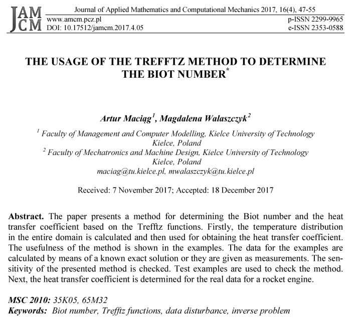
If the Trefftz functions for operator ![]() are known, the solution can be approximated by:
are known, the solution can be approximated by:
|
|
where ![]() are coefficients of the linear combination and
are coefficients of the linear combination and ![]() are Trefftz functions
for linear operator
are Trefftz functions
for linear operator ![]() . The coefficients of
the linear combination are calculated based on known initial and boundary
conditions. For this purpose a suitable functional, which describes the error
of fulfilling the initial and boundary conditions by
approximate solution in least square sense, has to be minimized. After
obtaining the temperature distribution in the entire domain, the heat transfer
coefficient can be calculated using the Robin boundary condition.
. The coefficients of
the linear combination are calculated based on known initial and boundary
conditions. For this purpose a suitable functional, which describes the error
of fulfilling the initial and boundary conditions by
approximate solution in least square sense, has to be minimized. After
obtaining the temperature distribution in the entire domain, the heat transfer
coefficient can be calculated using the Robin boundary condition.
3. Example of the problem with the data disturbance
The method presented in this article is illustrated by a suitable example. To check the quality of the approximation, test problems were chosen for which the exact solutions are known.
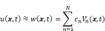
Let us consider the one dimensional heat conduction equation:
|
|
with initial and boundary conditions:
| (6) |
| (7) |
Moreover, the values of the temperature in 11
instants on the border ![]() = 0 for the
time between 6 and 16 seconds are known. They are called the internal
responses. In this example, the values of the internal responses were
calculated by means of an exact solution. In practice, they are given as
measurements.
= 0 for the
time between 6 and 16 seconds are known. They are called the internal
responses. In this example, the values of the internal responses were
calculated by means of an exact solution. In practice, they are given as
measurements.
The exact solution of a given problem is known and has a form:
| (8) |
In this case, the inverse problem is
considered (two conditions for ![]() = 0 and lack
of condition for
= 0 and lack
of condition for ![]() = 1).
For numerical simulation, the exact solution has been taken into account.
= 1).
For numerical simulation, the exact solution has been taken into account.
The presented problem was solved by the Trefftz method. There are several methods of determining the Trefftz function. In this case, the Trefftz functions are heat polynomials. They were introduced in [2, 3]. The first 8 Trefftz functions are as follows:
![]()
![]()
![]()
![]()
|
|
|
![]()
![]()
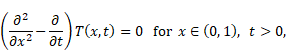
To determine the coefficients of the linear combination ![]() , the following
functional should be minimized:
, the following
functional should be minimized:
 |
After obtaining the temperature distribution in the entire domain, we can calculate the Biot number using the Robin condition in the form:
|
|
|
We can also obtain the value of the heat transfer coefficient using its relationship with the Biot number:
|
|
|
where ![]() is the heat transfer coefficient,
is the heat transfer coefficient, ![]() is the Biot number,
is the Biot number, ![]() is thermal conductivity
and
is thermal conductivity
and ![]() is characteristic
length.
is characteristic
length.
Generally, problems based on measurement data
can be very sensitive to the disturbance of the input data. The measurement
errors are usually the result of
interpolation of measuring instruments, the uncertainty associated with the
calibration and fluctuations in the sensor reading during the measurement.
Therefore,
the data disturbance sensitivity of the presented method has to be checked. Let
us assume that the internal responses ![]() are disturbed by a
random error
are disturbed by a
random error ![]() , which has a normal
distribution with a mean equal to 0 and a standard deviation
of 0.01, 0.02, 0.05, 0.07 and 0.09:
, which has a normal
distribution with a mean equal to 0 and a standard deviation
of 0.01, 0.02, 0.05, 0.07 and 0.09:
| (12) |
This means that the average disturbance of the data is at the level of 1, 2, 5, 7 and 9% respectively.
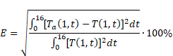
Because the exact solution is known, the
quality of the approximation of the boundary condition ![]() = 1 can be checked by calculating a mean relative error:
= 1 can be checked by calculating a mean relative error:
|
|
where ![]() is the approximate
solution and
is the approximate
solution and ![]() is the exact solution.
The values of the errors with and without the disturbance data depending on the
number of heat polynomials used in approximation are presented in Table 1.
is the exact solution.
The values of the errors with and without the disturbance data depending on the
number of heat polynomials used in approximation are presented in Table 1.
Table 1
A mean relative error of the boundary temperature approximation [%] depending on the number of the Trefftz functions and standard deviation
|
Number of functions |
Mean relative error [%] |
|||||
|
Exact data |
Disturbed data (standard deviation) |
|||||
|
0.01 |
0.02 |
0.05 |
0.07 |
0.09 |
||
|
5 6 7 8 |
2.59% 0.84% 0.21% 0.07% |
2.46% 1.06% 0.89% 4.309% |
5.09% 4.21% 3.71% 4.13% |
8.94% 11.67% 9.01% 10.95% |
11.53% 16.65% 12.55% 15.49% |
14.12% 21.63% 16.09% 20.05% |
Clearly, the Trefftz method gives very good results. In general, more Trefftz functions lead to better results. In this problem, the error of approximation is very small even for a small number of functions. The further increase in the number of heat polynomials causes an accumulation of numerical errors and worse results. Generally, for disturbed data the error is bigger. However, it should be noted that the disturbances of the internal responses do not cause a considerable increase of the error. Of course, greater disturbance results in bigger errors. The values presented in Table 1 show that even for a disturbance of 2%, the errors are on the level of 4%. For greater disturbance, the errors do not exceed a double disturbance. In the case where there is no disturbance of the data, the best results are obtained for 8 Trefftz functions and in the case where we consider the disturbance for 5 or 7 functions.
4. Example of the problem with the experimental data
The second example shows the usage of the
presented method for calculating the heat transfer coefficient and the Biot
number using experimental data. They concern the measurement of temperature on
the outer wall of the divergent nozzle rocket engine, made during testing of
the engine. The nozzle of the rocket engine
is responsible for the conversion of pressure resulting in a jet propulsion
engine. The nozzle is designed to increase the speed of gases produced
in the combustion process and the ejection of them which generates kinetic
energy to drive the rocket. In the divergent part of the nozzle, exhaust gases
during the expansion are additionally accelerated to supersonic speed, which
significantly increases the engine power. The wall thickness of the nozzle ![]() = 0.0211 m enables us to treat it as
an approximately flat slab.
= 0.0211 m enables us to treat it as
an approximately flat slab.
Therefore, let us consider the equation:
|
|

The equation should be completed by the initial boundary conditions:
| (15) |
| (16) |
Additionally, we know the temperature on the outer wall of the divergent nozzle rocket engine in 11 instants for the time between 6 and 16 seconds:
| (17) |
Other necessary data are as follows: the
ambient temperature of the nozzle ![]() = 300 K,
gas temperature in the nozzle
= 300 K,
gas temperature in the nozzle ![]() = 2946.2 K,
density
= 2946.2 K,
density ![]() = 7900 kg/m3,
specific heat
= 7900 kg/m3,
specific heat ![]() = 545
J/kgK, thermal conductivity
= 545
J/kgK, thermal conductivity ![]() = 35 W/mK.
= 35 W/mK.
This problem resembles the previous example but is based on the measurement data. Therefore it has been solved by means of Trefftz functions, as shown in the example above. After obtaining the temperature distribution in the entire domain, the Biot number was calculated using the formula:
|
|
|
Since in the first example the smallest errors were observed for 8 Trefftz functions, to solve the second problem, 8 heat polynomials have also been used.
This problem has been solved by many researchers using a variety of methods. The obtained values of the heat transfer coefficient by different methods are presented in Table 2.
In Table 2, the results obtained using the first five methods have been taken from literature. Methods 1 and 2 were presented by Grysa in [5]. The results of the third method are taken from Bartz article [6]. Mehta in papers [7] and [8] presented the results of methods 4 and 5 respectively. The last column shows the results obtained by the Trefftz method for 8 heat polynomials.
When comparing different methods we can see a relatively large variation of the results. This is probably related to the specifics of each method, meaning certain simplifications and calculation methods. The results obtained by the presented method seem to be correct in the physical sense. The value of the heat transfer coefficient increases with increasing temperature. There is no such relationship in the case of the methods 1, 3 and 4. In beginning of the first method, the heat transfer coefficient increases and then starts to decrease after 12 seconds. The third method is characterized by a constant value of the coefficient which probably results from the accepted model simplifications. A decrease in the heat transfer coefficient with increasing temperature seems even more incorrect. In the second method, we observe an increase in the coefficient value and then stabilization after 12 seconds at the level of 1130 W/m2K. In the fifth method, there is a similar trend as in the case of the Trefftz method, but the results obtained by the Trefftz method are about two times greater. If we take into consideration a mean of methods 1, 2, 3, 4 and 5 we obtain the values similar to the Trefftz method. A big advantage of the Trefftz method is the fact that the approximate solution strictly satisfies the governing equation.
Table 2
The values of the heat transfer coefficient obtained by various methods
|
Time [s] |
Temperature [K] |
Heat transfer
coefficient |
||||||
|
Other methods |
Trefftz method |
|||||||
|
1 |
2 |
3 |
4 |
5 |
Mean of methods 1, 2, 3, 4, 5 |
|||
|
6 7 8 9 10 11 12 13 14 15 16 |
324.69 342.02 355.99 379.92 402.01 425.01 440.01 459.99 478.99 507.01 527.97 |
738.8 1074.2 1175.7 1241.7 1291.6 1318.9 1300.4 1279.6 1257.6 1255.2 1248.5 |
239.5 696.6 884.3 969.5 1056.9 1111.7 1138.5 1133.6 1129.0 1127.0 1135.5 |
2254.2 2254.2 2254.2 2254.2 2254.2 2254.2 2254.2 2254.2 2254.2 2254.2 2254.2 |
1821.9 1810.0 1610.3 1690.9 1669.7 1641.9 1497.6 1443.1 1387.0 1413.0 1383.7 |
536.6 600.6 592.6 674.2 712.9 737.4 718.2 723.6 723.0 753.6 758.3 |
1118.2 1287.12 1303.42 1366.1 1397.06 1412.82 1381.78 1366.82 1350.16 1360.6 1356.04 |
953.3 993.2 1036.4 1083.3 1134.0 1189.0 1248.5 1313.1 1383.3 1459.5 1542.5 |
If we know the value of the heat transfer coefficient in subsequent moments of time, we can use formula (11) to calculate the value of the Biot number. Figure 1 shows the relationship between the heat transfer coefficient and the Biot number.
a) b)
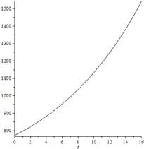
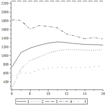
Fig. 1. The dependence of the heat transfer coefficient on time for Trefftz method (a) and for other methods (b)
In the analyzed example, the dependence of the heat transfer coefficient and the Biot number from time is characterized by the same shape. However, the values of the Biot number are about 1650 times lower than the values of the heat transfer coefficient. The Trefftz method gives a more regular graph than other methods.
5. Conclusions
The Trefftz method is very useful for many theoretical and practical problems of heat transfer. It gives very good results in the case of inverse problems, also concerning the identification of coefficients. It allows us to calculate the heat transfer coefficient and the Biot number when it is not possible to measure surface temperature, or when the measurement is very difficult.
A big advantage of this method is its mathematical simplicity. Moreover, the solution seems to be insensitive to data disturbance, which is very important if we solve problems based on measurements. In the first examples the results for disturbed data is of course worse than in the case of exact date. However the error stays at a level similar to a given disturbance. This method is also very effective even in the case of incomplete input data. In the presented examples the temperature measurements are given only for a certain period of time from 6 to 16 seconds. Using the described method, the error of approximation of the Biot number stays at a low level. For the example presented in the paper the approximation of the exact solution was highly satisfactory for a small number of heat polynomials. In the case of exact data, the best results are obtained for 8 Trefftz functions. When we consider noisy data the best results we get using 5 and 7 functions. The problem described in section 4 shows that the Trefftz method gives similar results to other methods presented in literature. It is very important that approximation obtained using Trefftz method strictly satisfies the governing equation. Therefore, the results seem to be more correct in physical sense.
References
[1] Trefftz E., Ein Gegenstueuk zum Ritz'schen Verfahren, Proceedings 2nd International Congres of Applied Mechanics, Zurich 1926, 131-137.
[2] Rosenbloom P.C., Widder D.V., Expansion in terms of heat polynomials and associated functions, Transactions of the American Mathematical Society 1956, 92, 220-266.
[3] Ciałkowski M.J., Frąckowiak A., Heat Functions and Their Application for Solving Heat Transfer and Mechanical Problems, Poznań University of Technology Publishers, Poznań 2000.
[4] Hożejowska S., Kaniowski R., Poniewski M.E., Application of adjustment calculus to the Trefftz method for calculating temperature field of the boiling liquid flowing in a minichannel, International Journal of Numerical Methods for Heat and Fluid Flow 2014, 24, 4, 811-824.
[5] Grysa K., Metody określania liczby Biota i współczynnika przejmowania ciepła, Journal of Theoretical and Applied Mechanics 1982, 20, 71-86.
[6] Bartz D.R., A simple equation for rapid estimation of rocket nozzle convective heat transfer coefficients, Jet Propulsion 1957, 49-51.
[7] Mehta R.C., Solution of the inverse conduction problem, AIAA Journal 1977, 1355-1356.
[8] Mehta R.C., Extention of the solution of inverse conduction problem, International Journal of Heat and Mass Transfer 1979, 1149-1150.
* This topic was presented at the conference Numerical Heat Transfer in Warsaw, 27-30 September 2015.