Pressure stabilized finite elements simulation for steady and unsteady Newtonian fluids
Ahmed Elhanafy
,Amr Guaily
,Ahmed Elsaid
Journal of Applied Mathematics and Computational Mechanics |
 Download Full Text |
PRESSURE STABILIZED FINITE ELEMENTS SIMULATION FOR STEADY AND UNSTEADY NEWTONIAN FLUIDS
Ahmed Elhanafy1, Amr Guaily2, Ahmed Elsaid1
1Mathematics & Engineering Physics
Department, Faculty of Engineering, Mansoura University
PO 35516, Mansoura, Egypt
2Engineering Mathematics & Physics Department, Faculty of
Engineering, Cairo University
PO 12613, Giza, Egypt
eng_hanafy2012@yahoo.com; amr.guaily@cu.edu.eg; a_elsaid@mans.edu.eg
Received: 24 November 2016; Accepted: 2 August 2017
Abstract. A numerical simulation of an incompressible viscous flow using the finite element method is presented. In this study, the pressure stabilization technique is suggested for the treatment of the incompressibility constraint for both steady and unsteady flow cases. To the best of the authors’ knowledge, the pressure stabilization technique is used for steady flows only. The proposed technique allows for equal low-order interpolation polynomials to be used for all variables which circumvent the so-called LBB compatibility condition without pressure checker boarding and solution instabilities. Results are obtained for two benchmark problems, namely, lid-driven cavity flow and the vortex-shedding behind a circular cylinder. The results are compared with published numerical and experimental works with an apparent degree of success.
MSC 2010:35Q30, 65M08, 65N08, 74S10, 76D05, 76M12
Keywords: unsteady incompressible viscous flow, pressure stabilization technique, equal low-order finite elements, Galerkin least squares
1. Introduction
The numerical simulation of unsteady incompressible flows is one of the most challenging topics since the continuity equation becomes a constraint equation for the velocity field rather than being an evolution equation for the density field. This problem appears when assuming incompressible fluids i.e. fluid with constant Lagrangian density and consequently the pressure does not affect the density. Differences in various methods of treating the incompressible flow equations originate from differences in strategies for satisfying the incompressibility constraint [1]. There are many methods for treating the incompressibility constraint in literature such as weakly incompressible solvers [2-4], the semi-implicit method for pressure-linked equations (SIMPLE) [5], the penalty formulation [6], the artificial compressibility formulation [7] and the pressure stabilization formulation [8]. Hughes [9] has suggested the penalty formulation for both steady and unsteady flow cases.
In this study, we adopt the pressure stabilization technique since equal order of interpolation functions for velocity and pressure can be used for finite element spatial discretization which is considered the main advantage of this formulation. This formulation is suggested and used by Habashi [10] for steady laminar viscous flows. The results in this work prove the validity of this technique for steady and unsteady flows with lower computational costs compared with the other traditional methods.
2. Governing equations
For non-polar Newtonian fluids with no heat or mass addition, conservation of linear momentum and mass for incompressible, unsteady, two-dimensional planar flows read
| (1) |
| (2) |
where ![]() is the density,
is the density,![]() is the velocity
vector,
is the velocity
vector,![]() is the isotropic
pressure and the stress tensor
is the isotropic
pressure and the stress tensor![]() is given by:
is given by:
![]() (3)
(3)
where ![]() is
the constant shear viscosity, and
is
the constant shear viscosity, and ![]() is the rate of the strain tensor given by:
is the rate of the strain tensor given by:
| (4) |
From a mathematical point of view, the
dimensionless formulation of the governing equation is preferable, so we use
the following non-dimensional scheme: ![]()
where ![]() is a
characteristic length,
is a
characteristic length, ![]() is the free stream velocity and
is the free stream velocity and ![]() is the free stream pressure. Omitting the asterisk (*) for
simplicity, the non-dimensional
Cartesian form of the governing equations can be written as:
is the free stream pressure. Omitting the asterisk (*) for
simplicity, the non-dimensional
Cartesian form of the governing equations can be written as:
| (5) |
| (6) |
![]() , (7)
, (7)
where ![]() and
and ![]() are
the horizontal and vertical velocity component respectively,
are
the horizontal and vertical velocity component respectively, ![]() is the physical time and Re is the Reynolds number defined as:
is the physical time and Re is the Reynolds number defined as:
![]() (8)
(8)
where![]() is the kinematic viscosity.
is the kinematic viscosity.
2.1. Pressure stabilization technique
In this formulation [8], the continuity equation is modified by adding a Laplacian term as follows:
![]() (9)
(9)
With this formulation, the conservation equations are coupled and the pressure checker boarding can be avoided. The main advantage of this formulation is the ability to use equal-order for interpolation functions for all variables which decreases the computational costs. See also [11] for more details.
3. Solution procedure
The standard Galerkin finite element method is used for the continuity equation since it is of an elliptic type while the GLS stabilization technique [12, 13] is used for the momentum equations since it is of a parabolic-hyperbolic type and consequently the convective terms need special treatment. Quadrilateral elements are chosen and all variables are interpolated by equal order bilinear shape functions. All integrals are evaluated numerically using the 3-point Gauss-Legender quadrature. The non-linear terms are linearized by average values of the velocity components over each element [14]. The Euler explicit scheme is used for time marching process. The time step is chosen in such a way to satisfy the CFL number to obtain a stable solution. Lumping approximation is applied to the consistent mass matrix converting it to a diagonal matrix [14]. The details are omitted sue to space limitations. See also [11] and [15] for more details.
4. Numerical results
The proposed formulation is applied to two benchmark problems. The first problem is the Lid-driven cavity flow and the second is the flow over circular cylinder. The governing equations are solved for different values of the Reynolds number and the results are compared with published numerical and experimental works.
4.1. Lid-driven cavity flow
The flow is confined in a unite square bounded by solid walls with a moving top boundary to the right. Due to the singularity of the flow field at the upper corners, we chose the regularized boundary condition for the upper wall which is given by the following relation:
| (10) |
The no-slip boundary condition for velocity components are imposed at the solid walls. Pressure is specified to be zero at the lower left corner point, with zero gradient over the walls. The Reynolds number is based on the side length of the cavity and the speed of the lid.
4.1.1. Results and discussion
The first simulation for this problem is
performed with clustered grid of
(40 x 40) elements to capture the high gradient near the walls as shown in
Figure 1. The Reynolds number is set to 100. For stability requirement, the
time step is taken as 0.0001 and the pressure dissipation parameter is![]() . The flow reaches the steady state after ten seconds with a total
number of iterations of 100000. Figures 2 and 3 show
the streamlines, the axial
. The flow reaches the steady state after ten seconds with a total
number of iterations of 100000. Figures 2 and 3 show
the streamlines, the axial ![]() component at x = 0.5 respectively which is compared with the work
of [2], [16] and [17] with an apparent degree of success.
component at x = 0.5 respectively which is compared with the work
of [2], [16] and [17] with an apparent degree of success.
The second simulation is performed for ![]() with the same mesh and the flow conditions. With the comparison of
the previous case, it is noted that the time required for obtaining the steady
state solution increases with the increase of the Reynolds number, as it takes
about 30 seconds. The corresponding streamlines and pressure contours are shown
in Figures 4 and 5, respectively. Along with the axial velocity at
with the same mesh and the flow conditions. With the comparison of
the previous case, it is noted that the time required for obtaining the steady
state solution increases with the increase of the Reynolds number, as it takes
about 30 seconds. The corresponding streamlines and pressure contours are shown
in Figures 4 and 5, respectively. Along with the axial velocity at![]() in
Figure 6. The results for this case are compared with the
results obtained in [13].
in
Figure 6. The results for this case are compared with the
results obtained in [13].
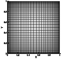
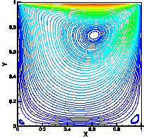
Fig. 1. Clustered 40 x 40 mesh Fig. 2. Steady streamlines at Re = 100
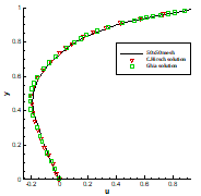
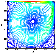
Fig. 3.![]() -comonent velocity at x = 0.5 Fig. 4. Steady
streamlines for Re = 1000
-comonent velocity at x = 0.5 Fig. 4. Steady
streamlines for Re = 1000
More solutions are obtained for this problem at a wide range of the Reynolds number values to show the effect of the Reynolds number on the primary vortex location and axial and normal velocities. The effect of Reynolds number can be also clearly seen from the axial and normal velocity components profiles at x = 0.5 and y = 0.5 as shown in Figures 7 and 8, respectively.
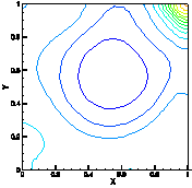
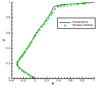
Fig. 5. Pressure contours for Re = 1000 Fig.
6. ![]() -comonent velocity at
-comonent velocity at![]() for
Re = 1000
for
Re = 1000
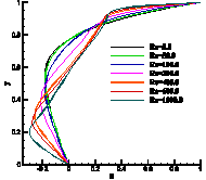
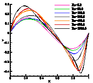
Fig. 7. Axial velocity at x = 0.5 Fig. 8. Normal velocity at y = 0.5
4.2. Flow over circular cylinder
One of the most challenging problems for numerical simulation of incompressible flows is the study of the flow over a circular cylinder. The dimensions of the computational domain are 20 and 9 cylinder diameters in the flow and cross-flow directions, respectively. The centre of the cylinder is located at a distance of 5 cylinder diameters from the inlet boundary and is located in the middle distance between the upper and lower boundaries. A clustered grid with a smaller element size near the cylinder wall is used as shown in Figure 9 with a total number of elements of 1200.
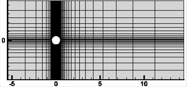
Fig. 9. Geometry and grid for the flow over cylinder problem
The initial conditions are zero velocity and
pressure everywhere. Uniform
velocity with a magnitude of 1 is specified at the inlet and normal derivative
of the ![]() -velocity component and
the
-velocity component and
the![]() -component itself are considered zero at the upper and lower
boundaries [14]. The Reynolds number is based on the inlet velocity and
cylinder diameter. The no-slip boundary condition for velocity components is
imposed on the cylinder surface. Neumann boundary condition for pressure is
imposed at the upper and the lower boundaries. At the exit boundary, the
pressure is fixed to be zero.
-component itself are considered zero at the upper and lower
boundaries [14]. The Reynolds number is based on the inlet velocity and
cylinder diameter. The no-slip boundary condition for velocity components is
imposed on the cylinder surface. Neumann boundary condition for pressure is
imposed at the upper and the lower boundaries. At the exit boundary, the
pressure is fixed to be zero.
4.2.1. Results and discussion
4.2.1.1. Steady state flow
The evolution of the flow eddies behind the cylinder is studied by varying the Reynolds number.
It is apparent that the pair of vortices symmetrically grows with the increase in the Reynolds number as shown in Figure 10. This fact can be shown clearly through the relation between the normalized reattachment length (S/D) and the Reynolds number, where S is the distance measured from the right end-point of the cylinder to the reattachment point where the two eddies end. The results obtained are compared with [2], [18] and [19] and summarized in Table 1. From the above results, it could be concluded that the pair of eddies grows almost linearly with the increase in the Reynolds number.
![]()
![]()
![]()
![]()
![]()
![]()
![]()
(a) Re = 20 (b) Re = 60
Fig. 10. The effect of increasing of Reynolds number on the length of the symmetric vortices
Table 1
Comparison of predicted reattachment length ratios (S/D)
|
Re |
Teneda [18] |
Xu et al. [2] |
Huang et al. [19] |
Present work |
|
25 |
1.15 |
1.12 |
.991 |
1.09 |
|
30 |
1.49 |
1.50 |
1.272 |
1.32 |
|
35 |
1.80 |
1.84 |
1.531 |
1.63 |
|
40 |
2.20 |
2.22 |
1.94 |
1.88 |
|
42 |
2.35 |
2.26 |
2.09 |
2.02 |
4.2.1.2. Time-dependent flow
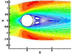
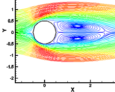
The solution for this case is obtained with Re = 100. For the stability requirement, the time step is set to 0.0005 and the pressure dissipation parameter is 0.005. Initially, a pair of symmetric attached vortices grew behind the cylinder. It is found that two vortices expand gradually with time increase which agrees with the experimental and numerical works in [14] and [20].
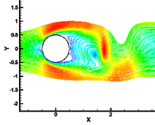
As time increases, small oscillations begin
to occur. To capture the vortex shedding, a perturbation is introduced in the
flow. This perturbation is inserted by changing the initial conditions by which
the flow enters vertically [21]. It takes about 50 seconds to capture the
vortex shedding which agrees with [14] and [20]. The observed period shedding
time![]() is 5.925 time units (corresponding to 11850 time steps), giving a
dimensionless shedding frequency, or Strouhal number
(St
is 5.925 time units (corresponding to 11850 time steps), giving a
dimensionless shedding frequency, or Strouhal number
(St ![]() ) of 1.687 compares well with the results of [14] and [20]. The
vortex shedding is shown using the streamlines and pressure contours for
different times in Figures 11 and 12, respectively.
) of 1.687 compares well with the results of [14] and [20]. The
vortex shedding is shown using the streamlines and pressure contours for
different times in Figures 11 and 12, respectively.
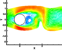
(a) Streamlines at ![]() (b) Streamlines at
(b) Streamlines at ![]()
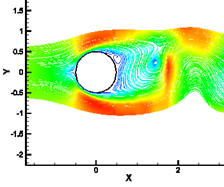
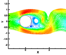
(c)
Streamlines at ![]() (d) Streamlines at
(d) Streamlines at ![]()
Fig. 11. Streamlines for different times of one cycle of the vortex shedding for Re = 100
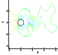
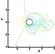
(a) Pressure contours at ![]() (b) Pressure contours at
(b) Pressure contours at ![]()
Fig. 12. Pressure contours for two different times of one cycle of the vortex shedding for Re = 100
5. Summary and conclusion
In this study, the pressure stabilized
technique is suggested for treating the
incompressibility constraint. The pressure
stabilization parameter ![]() is chosen to be in the order of the time step. The proposed technique circumvents the LBB computability
condition, stable solutions are obtained and equal-order interpolation
functions are used for all flow variables. A hybrid Galerkin Least-squares
finite
element/finite difference scheme is used in the discretization process. Two
benchmark problems, namely, lid-driven cavity flow and flow over circular
cylinder are considered. The results prove that the pressure stabilized
technique, usually used for steady flows only, can be also used for both steady
and unsteady flows.
is chosen to be in the order of the time step. The proposed technique circumvents the LBB computability
condition, stable solutions are obtained and equal-order interpolation
functions are used for all flow variables. A hybrid Galerkin Least-squares
finite
element/finite difference scheme is used in the discretization process. Two
benchmark problems, namely, lid-driven cavity flow and flow over circular
cylinder are considered. The results prove that the pressure stabilized
technique, usually used for steady flows only, can be also used for both steady
and unsteady flows.
For flow in the lid-driven cavity, results
are obtained for different values of the Reynolds number. The axial velocity
profile at x = 0.5 is compared with published works with an apparent
degree of agreement. The results assert that with the increase of the Reynolds
number, the main vortex moves down to the center of the cavity which is
consistent with the published experimental and computational works. For flow
over the circular cylinder, steady symmetric vortices at low Reynolds number
values i.e. ![]() are observed. It is noted that the length of the vortex increases
with the increase of the Reynolds number. The relation between the length of
the vortex and the Reynolds number is summarized. It is noted also that the
flow over the circular cylinder becomes time-dependent or periodic when the
Reynolds number is higher than 100. The vortex shedding is captured
successfully with the non-dimensional Strouhal number of 1.687 which agrees with the published computational results.
are observed. It is noted that the length of the vortex increases
with the increase of the Reynolds number. The relation between the length of
the vortex and the Reynolds number is summarized. It is noted also that the
flow over the circular cylinder becomes time-dependent or periodic when the
Reynolds number is higher than 100. The vortex shedding is captured
successfully with the non-dimensional Strouhal number of 1.687 which agrees with the published computational results.
References
[1] Kwak K., Kiris C., Chang J., Computational challenges of viscous incompressible flows, Journal of Computers and Fluids 2005, 34, 283-299.
[2] Xu G.X., Li E., Tan V., G.R. Liu, Simulation of steady and unsteady incompressible flow using gradient smoothing method(GSM), Journal of Computers and Structures 2012, 90-91, 131-144.
[3] Choi D., Merkle C., The application of preconditioning in viscous flows, Journal of Computational Physics 1993, 105, 203-226.
[4] Turkel E., Preconditioned methods for solving the incompressible and low speed compressible equations, Journal of Comput. Phys. 1987, 72, 277-375.
[5] Patankar S.V., Numerical Heat Transfer and Fluid Flow, Hemisphere Publishing, New York 1980.
[6] Courant R., Calculus of Variations and Supplementary Notes and Exercis, New York University, New York 1956.
[7] Chorin A.J., A numerical method for solving incompressible viscous flow problems, Journal of Computational Physics 1967, 212-226.
[8] Langtangen H.P., Mardal K., Winther R., Numerical methods for incompressible viscous flow, Journal of Advances in Water Resources 2002, 25, 1125-1146.
[9] Hughes T.J.R., Liu W.K., Brooks A., Finite element analysis of incompressible viscous flows by the penalty function formulation, Journal of Computational Physics 1979, 30, 1-60.
[10] Gunzburger M.D., Nicolaides R.A., Incompressible Computational Fluid Dynamics Trends and Advances, Cambridge University Press, 1993, 151-182.
[11] Elhanafy A., Study of blood flow in some arteries and veins using computational fluid dynamics, M.SC. thesis, Faculty of Engineering, Mansoura University, 2017.
[12] Hughes T.J.R., Franca L.P., Hulbert G.M., A new finite element formulation for computational fluid dynamics: VIII. The Galerkin/Least-squares method for advective-diffusive equations, Journal of Computer Methods in Applied Mechanics and Engineering 1989, 73, 173-189.
[13] Tezduyar T.E., Stabilized finite element formulations for incompressible flow computations, Journal of Advances in Applied Mechanics 1992, 28.
[14] Brooks A.N., Hughes T.J.R., Stremline upwind/Petrov-Galerkin formulations for convective dominated flows with particular emphasis on the incompressible Navier-Stokes equations, Journal of Computer Methods in Applied Mechanics and Engineering 1982, 32, 199-259.
[15] Elhanafy A., Guaily A., Esaid A., A hybrid stabilized finite element/finite difference method for unsteady viscoelastic flows, Journal of Mathematical modelling and Applications 2016, 2(1), 19-28.
[16] Hirsch C., Numerical Computation of Internal and External Flows, Vol. 1, Elsevier, 2007.
[17] Ghia U., Ghia K.N., Shin C.T., High-Re solutions for incompressible flow using the Navier- -Stokes equations and a multigrid method, Journal of Computer and Physics 1982, 48, 387-411.
[18] Teneda S., Experimental investigation of the wakes behind cylinders and plates at low Reynolds numbers, Journal of Physics Society 1956, 11(3), 302-309.
[19] Huang Y.Q., Deng J., Ren A.L., Research on lift and drag in unsteady viscous flow around circular cylinders, J. Zhejiang Univ. Sci. A 2003, 37(5), 596-601.
[20] Rahman M., Karim M., Abdul Alim M., Numerical investigation of unsteady flow past a circular cylinder using 2-D finite volume method, Journal of Naval Architecture and Marine Engineering 2007.
[21] Kasem T., Numerical simulation of incompressible oscillatory flow over rippled sea beds, M.SC. thesis, Faculty of Engineering, Cairo University, Elsevier, 2005.