Fractional heat conduction in multilayer spherical bodies
Stanisław Kukla
,Urszula Siedlecka
Journal of Applied Mathematics and Computational Mechanics |
 Download Full Text |
FRACTIONAL HEAT CONDUCTION IN MULTILAYER SPHERICAL BODIES
Stanisław Kukla, Urszula Siedlecka
Institute of Mathematics, Czestochowa
University of Technology
Częstochowa, Poland
stanislaw.kukla@im.pcz.pl, urszula.siedlecka@im.pcz.pl
Received: 29
September 2016; accepted: 02 November 2016
Abstract. In this paper an analytical solution of the time-fractional heat conduction problem in a spherical coordinate system is presented. The considerations deal the two-dimensional problem in multilayer spherical bodies including a hollow sphere, hemisphere and spherical wedge. The mathematical Robin conditions are assumed. The solution is a sum of time-dependent function satisfied homogenous boundary conditions and of a solution of the steady-state problem. Numerical example shows the temperature distributions in the hemisphere for various order of time-derivative.
Keywords: heat conduction, multilayer bodies, Caputo derivative, spherical coordinate
1. Introduction
The heat conduction in multilayer bodies with assumption of the Fourier law of heat transfer has been considered by Özişik in book [1]. Derivations of the temperature distributions in the bodies in rectangular, cylindrical and spherical coordinate systems were presented. The heat conduction in layered spheres with time-dependent boundary conditions assuming spherical symmetry was the subject of paper [2]. A solution of the heat conduction problem for a two-dimensional multi-layered sphere, hemisphere, spherical cone and spherical wedge presents paper [3].
A generalization of the Fourier law leads to a fractional heat conduction equation. The fractional differential equation governing the heat equation includes the fractional derivatives with respect to time and/or space variables. Properties of the fractional derivatives and methods to the solution of the fractional differential equations are presented in books [4-6]. A method of solution of a time-frac-tional heat conduction equation in a solid sphere has been discussed by Ning and Jiang in paper [7]. The time-fractional heat conduction in a multi-layered solid sphere assuming spherical symmetry was the subject of paper [8]. Heat conduction modelling using fractional order derivatives is presented by Žecová and J. Terpák in paper [9].
In this paper, an analytical solution of the time-fractional heat conduction for two-dimensional multilayered spherical bodies is presented. The condition for ensuring the perfect contact at interfaces and the mathematical Robin boundary conditions at boundary surfaces are assumed.
2. Formulation of the problem
Consider n spherical concentric layers
which are in perfect thermal contact.
The i-th layer (![]() ) occupied a region described by the spherical coordinates:
) occupied a region described by the spherical coordinates: ![]() ,
, ![]() (
(![]() ),
), ![]() ,
where
,
where ![]() is the radial coordinate,
is the radial coordinate,
![]() is the polar angle and
is the polar angle and ![]() is the azimuthal angle (Fig. 1).
is the azimuthal angle (Fig. 1).
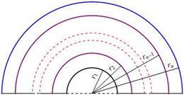
Fig. 1. A schematic diagram of the n-layered hemisphere
We suppose
that the i-th layer is characterized by constant thermal conductivity ![]() and constant thermal
diffusivity
and constant thermal
diffusivity ![]() . Moreover, assuming that the temperature doesn’t depend on
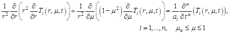
the azimuthal angle, the time fractional heat conduction
in the layers is governed by the following differential equation [10]:
. Moreover, assuming that the temperature doesn’t depend on
the azimuthal angle, the time fractional heat conduction
in the layers is governed by the following differential equation [10]:
| (1) |
where ![]() denotes fractional
order of the Caputo derivative with respect to time
denotes fractional
order of the Caputo derivative with respect to time ![]() ,
, ![]() . The Caputo derivative is defined by
[11]
. The Caputo derivative is defined by
[11]
| (2) |
In order
to simplify the equation (1) we introduce a new variable ![]() which is
related to the polar angle
which is
related to the polar angle ![]() by
by
| (3) |
Taking into account this relationship in equation (1) we obtain
 | (4) |
where ![]() . The differential equations (4) are complemented by boundary conditions
and the conditions providing the perfect thermal contact of the neigh-bouring
layers. The mathematical conditions are [2, 10]
. The differential equations (4) are complemented by boundary conditions
and the conditions providing the perfect thermal contact of the neigh-bouring
layers. The mathematical conditions are [2, 10]
| (5) |
| (6) |
| (7) |
| (9) |
where ![]() are inner and outer
heat transfer coefficients and
are inner and outer
heat transfer coefficients and ![]() are inner
and outer ambient temperatures. The initial condition is assumed in the form
are inner
and outer ambient temperatures. The initial condition is assumed in the form
| (10) |
3. Solution of the problem
We search a solution to the problem (1), (4)-(10) in the form of a sum
| (11) |
where the function ![]() satisfies
homogeneous fractional heat conduction
differential equation and homogeneous boundary conditions and the function
satisfies
homogeneous fractional heat conduction
differential equation and homogeneous boundary conditions and the function ![]() is a solution of a steady-state problem. Substituting the solution
(11) into equations (1), (4)-(10) we obtain the problems for the
functions
is a solution of a steady-state problem. Substituting the solution
(11) into equations (1), (4)-(10) we obtain the problems for the
functions ![]() and
and ![]() . For
. For
![]() we have
we have
| (12) |
| (13) |
| (14) |
| (15) |
| (16) |
| (17) |
| (18) |
The functions ![]() satisfy
the following boundary problem
satisfy
the following boundary problem
| (19) |
| (20) |
| (21) |
| (22) |
| (23) |
| (24) |
3.1. Solution to the homogeneous problem
We find
the time dependent function ![]() as a solution of the problem (12)-(18), by using the separation
of variables method. Substituting the product of functions
as a solution of the problem (12)-(18), by using the separation
of variables method. Substituting the product of functions
| (25) |
into equation (12), we obtain three differential equations
| (26) |
| (27) |
| (28) |
where![]() ,
, ![]() and
and ![]() are
separation constants.
are
separation constants.
Solution of the equation (26)
Assuming
that ![]() , the general solution of equation (26) can
be
written in the form
, the general solution of equation (26) can
be
written in the form
| (29) |
where ![]() and
and ![]() are the Legendre functions of order
are the Legendre functions of order ![]() . Because
. Because ![]() ,
we assume
,
we assume ![]() . Taking into account that
. Taking into account that
| (30) |
and
substituting function ![]() in the form (25) into equation (15), we
obtain an eigenvalue equation
in the form (25) into equation (15), we
obtain an eigenvalue equation
| (31) |
Solving
equation (31a) or (31b), we obtain a sequence of roots ![]() .
The functions
.
The functions ![]() corresponding to the values of
corresponding to the values of ![]() create an orthogonal
system of functions, i.e. the functions satisfy the orthogonality
condition
create an orthogonal
system of functions, i.e. the functions satisfy the orthogonality
condition
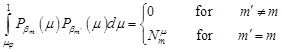 | (32) |
Solution of the equation (27)
The general solution of equation (27) has the form
| (33) |
where ![]() and
and ![]() are spherical Bessel functions of the first and second kind,
respectively. Substituting function
are spherical Bessel functions of the first and second kind,
respectively. Substituting function ![]() into
equation (25) and next, the obtained function
into
equation (25) and next, the obtained function ![]() into
conditions (13)-(14) and (16)-(17), the system of
into
conditions (13)-(14) and (16)-(17), the system of ![]() homogeneous equations is received. We rewrite the equation system in the matrix
form
homogeneous equations is received. We rewrite the equation system in the matrix
form
| (34) |
where ![]() and
and ![]() .
.
The non-zero solutions of equation (34) exist
for these values of ![]() for which the determinant of
the matrix
for which the determinant of
the matrix ![]() disappears, i.e.
disappears, i.e.
| (35) |
Solving this equation for ![]() , the sequences of
, the sequences of ![]() are obtained. For each value of
are obtained. For each value of ![]() , the coefficients
, the coefficients ![]() occurring in equation (33) are
determined by solving equation (34). The functions
occurring in equation (33) are
determined by solving equation (34). The functions ![]() corresponding
to the values of
corresponding
to the values of ![]() satisfy the orthogonality
condition
satisfy the orthogonality
condition
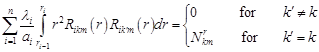 | (36) |
Solution of the equation (28)
Based on the orthogonality conditions (32),
(36) and using (25) in the condition (18), we find the initial condition for
the function ![]()
 | (37) |
The solution of the fractional differential equation (28) satisfying the initial condition (37) has the form
 | (38) |
where ![]() is Mittag-Leffler function [12].
is Mittag-Leffler function [12].
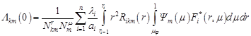
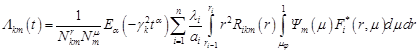
Ultimately, using (25), (30), (33) and (38), we have
| (39) |
where ![]() is given by equation
(38).
is given by equation
(38).
3.2. Solution to the steady-state problem
We seek a solution of the problem (19)-(24) in the form of a series
| (40) |
where ![]() are roots
of the equation (31a) or (31b). Substituting the
function
are roots
of the equation (31a) or (31b). Substituting the
function ![]() into equation (19) we obtain an Euler
differential equation
into equation (19) we obtain an Euler
differential equation
| (41) |
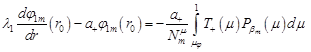
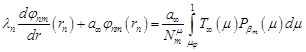
Next, taking into
account function (40) in equations (20)-(21) and (23)-(24) and
using the orthogonality condition (32), the boundary conditions for the
functions ![]() are obtained
are obtained
 | (42) |
 | (43) |
| (44) |
| (45) |
The general solution of the Euler equation (41) has the form
![]() (46)
(46)
Substitution
(46) in conditions (42)-(45) gives ![]() linear
non-homogeneous
equations which can be written in the matrix form
linear
non-homogeneous
equations which can be written in the matrix form
![]() (47)
(47)
where ![]() ,
, ![]() and
and ![]() .
The equation (47) is than solved with respect to unknown
.
The equation (47) is than solved with respect to unknown ![]() . The determined
coefficients
. The determined
coefficients ![]() are then used in equation
(46). Thus, the function
are then used in equation
(46). Thus, the function ![]() as a solution of the
steady-state problem is given by equation (40) where the functions
as a solution of the
steady-state problem is given by equation (40) where the functions ![]() are defined by equation (46).
are defined by equation (46).
Finally, the temperature distribution in the spherical layers received on the basis of the fractional heat conduction model is given by equation (11), (39) and (40).
4. Numerical example
We use the
solution of the heat conduction problem derived in Section 3 to
numerical calculations of the temperature distribution in a layered hemisphere (![]() ). We assume that zero temperature is
established at the surface
). We assume that zero temperature is
established at the surface ![]() ,
i.e. the boundary conditions (15a) and (22a),
are satisfied. The considered hemisphere consists of five concentric layers
whose locations are determined by
non-dimensional radii:
,
i.e. the boundary conditions (15a) and (22a),
are satisfied. The considered hemisphere consists of five concentric layers
whose locations are determined by
non-dimensional radii: ![]() , where
, where ![]() . The non-dimensional radii
. The non-dimensional radii ![]() , thermal conductivity
, thermal conductivity ![]() and thermal diffusivity
and thermal diffusivity ![]() in the i-th layer of the sphere
are:
in the i-th layer of the sphere
are: ![]() ,
, ![]() ,
, ![]() , i = 1,…,5. The inner and outer heat
transfer coefficients are:
, i = 1,…,5. The inner and outer heat
transfer coefficients are: ![]() ,
the inner and outer ambient temperatures are:
,
the inner and outer ambient temperatures are: ![]() and
the initial temperature is assumed as constant:
and
the initial temperature is assumed as constant: ![]() . The
computations were performed for various values of the order of fractional
time-derivative:
. The
computations were performed for various values of the order of fractional
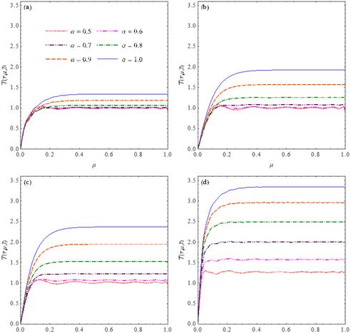
time-derivative: ![]() . The temperature
distributions on the surfaces of the layers determined for
. The temperature
distributions on the surfaces of the layers determined for ![]() , are shown in Figures 2a-d. The
temperature depends on the order
, are shown in Figures 2a-d. The
temperature depends on the order ![]() of the
time-derivative occurring in the heat conduction model. This dependence is more
significant for higher temperature of the sphere.
of the
time-derivative occurring in the heat conduction model. This dependence is more
significant for higher temperature of the sphere.
![]()
Fig. 2. The
non-dimensional temperatures at outer surface and at interfaces of the layered
hemisphere: a) ![]() , b)
, b) ![]() , c)
, c) ![]() , d)
, d) ![]()
5. Conclusions
An analytical solution of the problem of time-fractional heat conduction in two-dimensional multi-layer spherical bodies has been presented. The formulation of the problem includes the heat conduction in the spherical bodies which occupied regions defined by finite intervals of the radial coordinate and polar angle. The conditions to perfect contact at interfaces and the mathematical Robin boundary conditions were assumed. The derived solution applies to the bodies consisting of an arbitrary number of layers which are characterized by different thermal conductivity and thermal diffusivity. The numerical example shows that the order of fractional time-derivative is of significant importance for temperature distribution in the body. The temperature at the outer surface and at interfaces of the layered hemisphere is lower order of the fractional time-derivative. The further research will take into consideration the fractional heat conduction in spherical multilayer bodies with time-dependent boundary conditions.
References
[1] Özişik M.N., Heat conduction, Wiley, New York 1993.
[2] Lu X., Viljanen M., An analytical method to solve heat conduction in layered spheres with time-dependent boundary conditions, Physics Letters A 2006, 351, 274-282.
[3] Jain P.K., Singh S., Rizwan-uddin, An exact analytical solution for two-dimensional, unsteady, multilayer heat conduction in spherical coordinates, International Journal of Heat and Mass Transfer 2010, 53, 2133-2142.
[4] Diethelm K., The Analysis of Fractional Differential Equations, Springer-Verlag, Berlin Heidelberg 2010.
[5] Podlubny I., Fractional Differential Equations, Academic Press, San Diego 1999.
[6] Povstenko Y., Linear Fractional Diffusion-wave Equation for Scientists and Engineers, Birkhäuser, New York 2015.
[7] Ning T.H., Jiang X.Y., Analytical solution for the time-fractional heat conduction equation in spherical coordinate system by the method of variable separation, Acta Mechanica Sinica 2011, 27(6), 994-1000.
[8] Kukla S., Siedlecka U., An analytical solution to the problem of time-fractional heat conduction in a composite sphere, Bulletin of the Polish Academy of Sciences, Technical Sciences (in print).
[9] Žecová M., Terpák J., Heat conduction modeling by using fractional-order derivatives, Applied Mathematics and Computation 2015, 257, 365-373.
[10] Povstenko Y., Fractional heat conduction in an infinite medium with a spherical inclusion, Entropy 2013, 15, 4122-4133.
[11] Ishteva M., Scherer R., Boyadjiev L., On the Caputo operator of fractional calculus and C-Laguerre functions, Mathematical Sciences Research Journal 2005, 9(6), 161-170.
[12] Haubold H.J., Mathai A.M., Saxena R.K., Mittag-Leffler functions and their applications, Journal of Applied Mathematics, Article ID 298628, 2011.